A ChannelTS object is a container for a single channel. The data are stored in an xarray.DataArray and indexed by time according to the metadata provided. Here we will make a simple electric channel and look at how to interogate it.
To get a ChannelTS object from an MTH5 file you can use
ch_dataset = mth5_object.get_channel("station", "run", "ex", survey="survey")
ch_ts = ch_dataset.to_channel_ts()
%matplotlib inline
import numpy as np
from mth5.timeseries import ChannelTS
from mt_metadata.timeseries import Electric, Run, StationCreate Synthetic ChannelTS
Here create some metadata, the keys are the time_period.start and the sample_rate.
ex_metadata = Electric()
ex_metadata.time_period.start = "2020-01-01T00:00:00"
ex_metadata.sample_rate = 1.0
ex_metadata.component = "ex"
ex_metadata.dipole_length = 100.
ex_metadata.units = "milliVolt"
Create Station and Run metadata
station_metadata = Station(id="mt001")
run_metadata = Run(id="001")
Create “realistic” data
n_samples = 4096
t = np.arange(n_samples)
data = np.sum([np.cos(2*np.pi*w*t + phi) for w, phi in zip(np.logspace(-3, 3, 20), np.random.rand(20))], axis=0)
ex = ChannelTS(channel_type="electric",
data=data,
channel_metadata=ex_metadata,
run_metadata=run_metadata,
station_metadata=station_metadata)exChannel Summary:
Survey: 0
Station: mt001
Run: 001
Channel Type: Electric
Component: ex
Sample Rate: 1.0
Start: 2020-01-01T00:00:00+00:00
End: 2020-01-01T01:08:15+00:00
N Samples: 4096Plot Timeseries
ex.plot()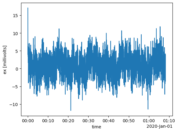
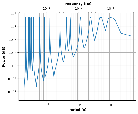
Plot Spectra
ex.plot_spectra()C:\Users\peaco\OneDrive\Documents\GitHub\mth5\mth5\timeseries\channel_ts.py:1634: RuntimeWarning: divide by zero encountered in divide
ax.loglog(1.0 / plot_frequency, power, lw=1.5)
Get a slice of the data
Here we will provide a start time of the slice and the number of samples that we want the slice to be
ex_slice = ex.get_slice("2020-01-01T00:00:00", n_samples=256)ex_sliceChannel Summary:
Survey: 0
Station: mt001
Run: 001
Channel Type: Electric
Component: ex
Sample Rate: 1.0
Start: 2020-01-01T00:00:00+00:00
End: 2020-01-01T00:04:15+00:00
N Samples: 256Plot Slice
ex_slice.plot()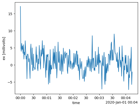
Downsample
Many times its advantageous to downsample the data for processing or visualization. There are a few methods for downsampling including
| Method | Description |
|---|---|
decimate | classic decimation: apply an anti-alias window then down sample by up to a factor of 8, if more are required repeat |
resample | no anti-alias filter just simply pick samples at the new sample rate |
resample_poly | upsampled, an FIR zero-phase low pass filter is applied then downsampled, efficient and most accurate preferred method |
ex_resample_poly = ex.resample_poly(.25)ex_resample_polyChannel Summary:
Survey: 0
Station: mt001
Run: 001
Channel Type: Electric
Component: ex
Sample Rate: 0.0
Start: 2020-01-01T00:00:00+00:00
End: 2020-01-01T01:08:12+00:00
N Samples: 1024ex_resample_poly.plot()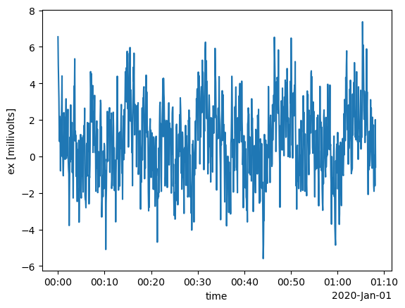
Convert to an xarray
We can convert the ChannelTS object to an xarray.DataArray which could be easier to use.
ex_xarray = ex.to_xarray()ex_xarrayex_xarray.plot()Convert to an Obspy.Trace object
The ChannelTS object can be converted to an obspy.Trace object. This can be useful when dealing with data received from a mainly seismic archive like IRIS. This can also be useful for using some tools provided by Obspy.
Note there is a loss of information when doing this because an obspy.Trace is based on miniSEED data formats which has minimal metadata.
ex.station_metadata.fdsn.id = "mt001"
ex_trace = ex.to_obspy_trace()
c:\Users\peaco\miniconda3\envs\py311\Lib\site-packages\obspy\core\util\attribdict.py:199: UserWarning: Attribute "network" must be of type <class 'str'>, not <class 'NoneType'>. Attempting to cast None to <class 'str'>
warnings.warn(msg)
ex_traceNone.MT001..LQN | 2020-01-01T00:00:00.000000Z - 2020-01-01T01:08:15.000000Z | 1.0 Hz, 4096 samplesConvert from an Obspy.Trace object
We can reverse that and convert an obspy.Trace into a ChannelTS. Again useful when dealing with seismic dominated archives.
ex_from_trace = ChannelTS()
ex_from_trace.from_obspy_trace(ex_trace)ex_from_traceChannel Summary:
Survey: 0
Station: MT001
Run: sr1_001
Channel Type: Electric
Component: ex
Sample Rate: 1.0
Start: 2020-01-01T00:00:00+00:00
End: 2020-01-01T01:08:15+00:00
N Samples: 4096exChannel Summary:
Survey: 0
Station: mt001
Run: 001
Channel Type: Electric
Component: ex
Sample Rate: 1.0
Start: 2020-01-01T00:00:00+00:00
End: 2020-01-01T01:08:15+00:00
N Samples: 4096On comparison you can see the loss of metadata information.
Logic
Overloads of some basic functionality are provided for ==, >, < and +.
Equals
This tests if the metadata and data are equal between two ChannelTS objects.
Here we are testing the original ex and the resampled ex, so they should not be equal. The logging messages provides information on which is not equal like the sampling rate and the end time.
ex == ex_resample_poly2025-09-24T22:15:39.722270-0700 | INFO | mt_metadata.base.metadata | __eq__ | sample_rate: 0.0 != 1.0
2025-09-24T22:15:39.722270-0700 | INFO | mt_metadata.base.metadata | __eq__ | time_period.end: 2020-01-01T01:08:12+00:00 != 2020-01-01T01:08:15+00:00
Falseother_ex = ex.copy()
other_ex.start = ex.end + 10
other_exChannel Summary:
Survey: 0
Station: mt001
Run: 001
Channel Type: Electric
Component: ex
Sample Rate: 1.0
Start: 2020-01-01T01:08:25+00:00
End: 2020-01-01T02:16:40+00:00
N Samples: 4096ex < other_ex2025-09-24T22:19:26.378242-0700 | INFO | mth5.timeseries.channel_ts | __lt__ | Only testing start time
FalseAdding Channels
Here we will add two channels ex and other_ex.
combined_ex = ex + other_ex
combined_ex
Channel Summary:
Survey: 0
Station: mt001
Run: 001
Channel Type: Electric
Component: ex
Sample Rate: 1.0
Start: 2020-01-01T00:00:00+00:00
End: 2020-01-01T02:16:40+00:00
N Samples: 8201combined_ex.plot()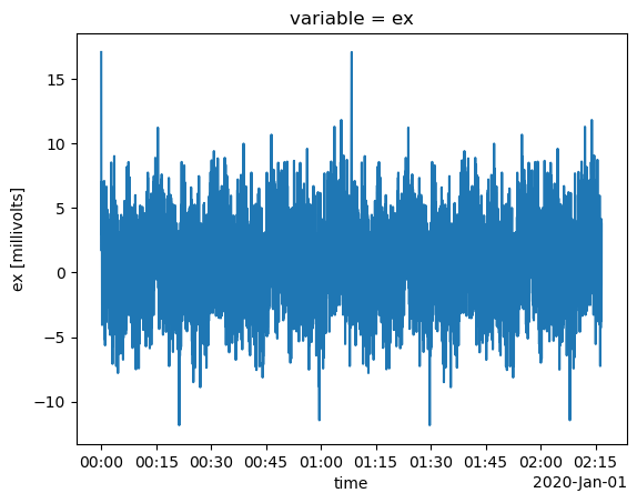
Merge
A different method for combining ChannelTS objects is to use the merge method. The advantage of using merge is that it provides a way to fill time gaps and resample as well.
resample_other_ex = ex.merge(
    other_ex,
    gap_method="slinear",
    new_sample_rate=0.5,
    resample_method="poly"
)

resample_other_ex.plot()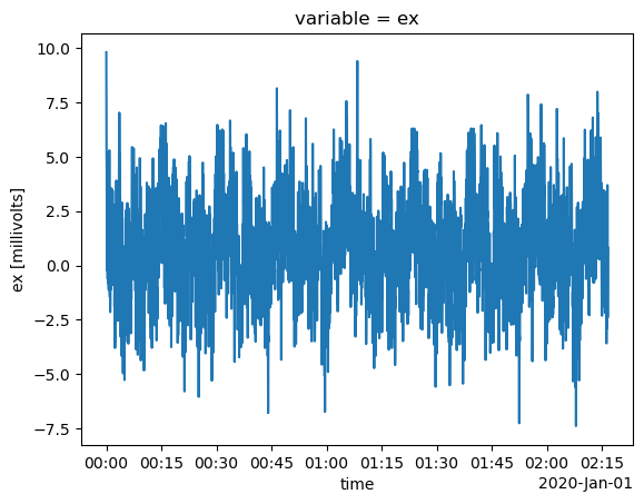
Calibrate
Removing the instrument response to calibrate the data is an important step in processing the data. A convenience function ChannelTS.remove_instrument_response is supplied just for this.
Currently, it will calibrate the whole time series at once and therefore may be slow for large data sets.
SEE ALSO: Make Data From IRIS examples for working examples.
help(ex.remove_instrument_response)Help on method remove_instrument_response in module mth5.timeseries.channel_ts:
remove_instrument_response(include_decimation=False, include_delay=False, **kwargs) method of mth5.timeseries.channel_ts.ChannelTS instance
Remove instrument response from the given channel response filter
The order of operations is important (if applied):
1) detrend
2) zero mean
3) zero pad
4) time window
5) frequency window
6) remove response
7) undo time window
8) bandpass
:param include_decimation: Include decimation in response,
defaults to True
:type include_decimation: bool, optional
:param include_delay: include delay in complex response,
defaults to False
:type include_delay: bool, optional
**kwargs**
:param plot: to plot the calibration process [ False | True ]
:type plot: boolean, default True
:param detrend: Remove linar trend of the time series
:type detrend: boolean, default True
:param zero_mean: Remove the mean of the time series
:type zero_mean: boolean, default True
:param zero_pad: pad the time series to the next power of 2 for efficiency
:type zero_pad: boolean, default True
:param t_window: Time domain windown name see `scipy.signal.windows` for options
:type t_window: string, default None
:param t_window_params: Time domain window parameters, parameters can be
found in `scipy.signal.windows`
:type t_window_params: dictionary
:param f_window: Frequency domain windown name see `scipy.signal.windows` for options
:type f_window: string, defualt None
:param f_window_params: Frequency window parameters, parameters can be
found in `scipy.signal.windows`
:type f_window_params: dictionary
:param bandpass: bandpass freequency and order {"low":, "high":, "order":,}
:type bandpass: dictionary