import numpy as np
from simpeg.electromagnetics import natural_source as nsem
from simpeg import maps
import matplotlib.pyplot as plt
import matplotlib
import matplotlib.gridspec as gridspec
from simpeg.utils import plot_1d_layer_model
from discretize import TensorMesh
from simpeg import (
    maps,
    data,
    data_misfit,
    regularization,
    optimization,
    inverse_problem,
    inversion,
    directives,
    utils,
)
from mtpy import MTCollection
mc = MTCollection()
mc.open_collection("../../data/transfer_functions/yellowstone_mt_collection.h5")
from ipywidgets import widgets, interact
station_names = mc.dataframe.station.values
def foo(name, component):
tf = mc.get_tf(name)
tf.plot_mt_response()
Q = interact(
foo,
name=widgets.Select(options=station_names, value='YNP05S'),
component=widgets.RadioButtons(options=['xy', 'yx', 'det'], value='xy')
)Loading...
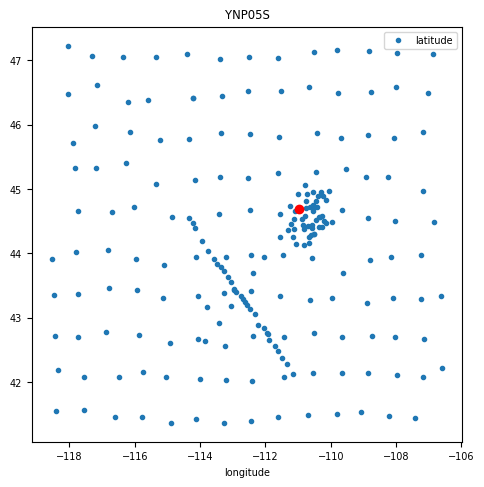
name = Q.widget.kwargs['name']
component = Q.widget.kwargs['component']
tf = mc.get_tf(name)

fig, ax = plt.subplots(1,1, figsize=(5,5))
mc.dataframe.plot(x='longitude', y='latitude', marker='.', linestyle='None', ax=ax)
ax.plot(tf.longitude, tf.latitude, 'ro')
ax.set_title(name)
24:10:30T22:26:20 | WARNING | line:311 |mtpy.core.mt_collection | get_tf | Found multiple transfer functions with ID YNP05S. Suggest setting survey, otherwise returning the TF from survey YSBB.
if component == 'xy':
    print ('>> Use Zxy')
    dobs = np.c_[tf.Z.res_xy, tf.Z.phase_xy].flatten()
    dobs_error = np.c_[tf.Z.res_error_xy, tf.Z.phase_error_xy].flatten()
elif component == 'yx':
    print ('>> Use Zyx')
    dobs = np.c_[tf.Z.res_yx, tf.Z.phase_yx].flatten()
    dobs_error = np.c_[tf.Z.res_error_yx, tf.Z.phase_error_yx].flatten()
elif component == 'det':
    print ('>> Use determinant')
    dobs = np.c_[tf.Z.res_det, tf.Z.phase_det].flatten()
    dobs_error = np.c_[tf.Z.res_error_det, tf.Z.phase_error_det].flatten()

frequencies = 1./tf.period
>> Use Zxy
tf.Z.z.real[:,0,0]array([-1.0593e+02, -9.2574e+01, -7.2999e+01, -5.9715e+01, -4.5300e+01,
-3.6534e+01, -2.7935e+01, -2.3598e+01, -1.8590e+01, -1.7163e+01,
-1.3645e+01, -1.2296e+01, -9.5656e+00, -7.9090e+00, -5.4159e+00,
-3.8748e+00, -2.0633e+00, -9.6175e-01, -2.0381e-01, 3.1078e-01,
2.5246e-01, 8.7086e-02, 5.3124e-01, 7.1696e-01, 5.9307e-01,
6.3013e-01, 4.9378e-01, 4.3698e-01, 3.2330e-01, 2.7804e-01,
2.2583e-01, 2.1039e-01, 1.1930e-01, 1.0868e-01, 5.8183e-02,
6.6387e-02, 2.0888e-02])tf.frequencyarray([2.5600e+02, 1.9200e+02, 1.2800e+02, 9.6000e+01, 6.4000e+01,
4.8000e+01, 3.2000e+01, 2.4000e+01, 1.6000e+01, 1.2000e+01,
8.0000e+00, 6.0000e+00, 4.0000e+00, 3.0000e+00, 2.0000e+00,
1.5000e+00, 1.0000e+00, 7.5000e-01, 5.0000e-01, 3.7500e-01,
2.5000e-01, 1.8750e-01, 1.2500e-01, 9.3750e-02, 6.2500e-02,
4.6875e-02, 3.1250e-02, 2.3438e-02, 1.5625e-02, 1.1719e-02,
7.8125e-03, 5.8594e-03, 3.9062e-03, 2.9297e-03, 1.9531e-03,
1.4648e-03, 9.7656e-04])dobsarray([358.90273828, 51.43326537, 340.34661177, 53.9133755 ,
302.42469781, 57.90557602, 269.34608354, 60.37133516,
221.96027781, 62.74461371, 189.95761582, 63.72680514,
152.88693152, 63.97985439, 133.76857224, 63.58541656,
105.95059052, 62.25563314, 95.92547857, 60.92500333,
77.011205 , 57.89460134, 69.94257313, 54.78715573,
62.9872013 , 48.970946 , 62.92421633, 44.61624917,
68.5985021 , 39.65404125, 75.7476336 , 37.27663258,
88.1884576 , 35.34609626, 97.08520987, 35.38513329,
113.08421156, 36.46588642, 117.82627586, 36.89441412,
138.89824131, 39.15962482, 150.27927762, 40.87831867,
151.41859042, 47.82852651, 148.12503966, 52.10125548,
125.19427549, 54.7742191 , 117.35936073, 58.25250697,
93.89116576, 61.77229208, 81.4369936 , 61.98162578,
65.47057318, 61.70010215, 60.06469253, 60.59230301,
50.15375403, 55.3470202 , 45.83228582, 53.68449207,
44.26012459, 50.54925441, 43.29136545, 47.94904011,
45.19637749, 47.84419407, 52.1403606 , 48.08811308,
53.48800944, 49.3715875 ])dz = 50
n_layer = 31
z_factor = 1.2
layer_thicknesses_inv = dz*z_factor**np.arange(n_layer-1)[::-1]def run_fixed_layer_inversion(
dobs,
standard_deviation,
rho_0,
rho_ref,
maxIter=10,
maxIterCG=100,
alpha_s=1e-10,
alpha_z=1,
beta0_ratio=1,
coolingFactor=2,
coolingRate=1,
chi_factor=1,
use_irls=False,
p_s=2,
p_z=2
):
mesh_inv = TensorMesh([(np.r_[layer_thicknesses_inv, layer_thicknesses_inv[-1]])], "N")
receivers_list = [
nsem.receivers.PointNaturalSource(component="app_res"),
nsem.receivers.PointNaturalSource(component="phase"),
]
source_list = []
for freq in frequencies:
source_list.append(nsem.sources.Planewave(receivers_list, freq))
survey = nsem.survey.Survey(source_list)
sigma_map = maps.ExpMap(nP=len(layer_thicknesses_inv)+1)
simulation = nsem.simulation_1d.Simulation1DRecursive(
survey=survey,
sigmaMap=sigma_map,
thicknesses=layer_thicknesses_inv,
)
# Define the data
data_object = data.Data(survey, dobs=dobs, standard_deviation=standard_deviation)
# Initial model
m0 = np.ones(len(layer_thicknesses_inv)+1) * np.log(1./rho_0)
# Reference model
mref = np.ones(len(layer_thicknesses_inv)+1) * np.log(1./rho_ref)
dmis = data_misfit.L2DataMisfit(simulation=simulation, data=data_object)
# Define the regularization (model objective function)
reg = regularization.Sparse(mesh_inv, alpha_s=alpha_s, alpha_x=alpha_z, reference_model=mref, mapping=maps.IdentityMap(mesh_inv))
print (reg.alpha_s, reg.alpha_z)
# Define how the optimization problem is solved. Here we will use an inexact
# Gauss-Newton approach that employs the conjugate gradient solver.
opt = optimization.InexactGaussNewton(maxIter=maxIter, maxIterCG=maxIterCG, tolG=1e-40, eps=1e-30)
# Define the inverse problem
inv_prob = inverse_problem.BaseInvProblem(dmis, reg, opt)
#######################################################################
# Define Inversion Directives
# ---------------------------
#
# Here we define any directives that are carried out during the inversion. This
# includes the cooling schedule for the trade-off parameter (beta), stopping
# criteria for the inversion and saving inversion results at each iteration.
#
# Defining a starting value for the trade-off parameter (beta) between the data
# misfit and the regularization.
starting_beta = directives.BetaEstimate_ByEig(beta0_ratio=beta0_ratio)
# Set the rate of reduction in trade-off parameter (beta) each time the
# the inverse problem is solved. And set the number of Gauss-Newton iterations
# for each trade-off paramter value.
beta_schedule = directives.BetaSchedule(coolingFactor=coolingFactor, coolingRate=coolingRate)
save_dictionary = directives.SaveOutputDictEveryIteration()
save_dictionary.outDict = {}
# Setting a stopping criteria for the inversion.
target_misfit = directives.TargetMisfit(chifact=chi_factor)
precond = directives.UpdatePreconditioner()
if use_irls:
reg.norms = np.r_[p_s, p_z]
reg.gradient_type = 'components'
# Reach target misfit for L2 solution, then use IRLS until model stops changing.
IRLS = directives.Update_IRLS(max_irls_iterations=100, minGNiter=1, f_min_change=1e-5)
IRLS.coolEpsFact = 1.5
precond = directives.UpdatePreconditioner()
# The directives are defined as a list.
directives_list = [
IRLS,
starting_beta,
save_dictionary,
precond
]
else:
# The directives are defined as a list.
directives_list = [
starting_beta,
beta_schedule,
target_misfit,
save_dictionary
]
#####################################################################
# Running the Inversion
# ---------------------
#
# To define the inversion object, we need to define the inversion problem and
# the set of directives. We can then run the inversion.
#
# Here we combine the inverse problem and the set of directives
inv = inversion.BaseInversion(inv_prob, directives_list)
# Run the inversion
recovered_model = inv.run(m0)
return recovered_model, save_dictionary.outDictrelative_error_rho = 0.05
floor_phase = 2.
rho_app = dobs.reshape((len(frequencies), 2))[:,0]
phase = dobs.reshape((len(frequencies), 2))[:,1]
standard_deviation = np.c_[abs(rho_app)*relative_error_rho, np.ones(len(phase))*floor_phase].flatten()
# standard_deviation += dobs_error
rho_0 = 100
rho_ref = 100.Run Smooth L2-norm inversion
recovered_model, output_dict = run_fixed_layer_inversion(
    dobs,
    standard_deviation,
    rho_0,
    rho_ref,
    maxIter=10,
    maxIterCG=30,
    alpha_s=1e-10,
    alpha_z=1,
    beta0_ratio=1,
    coolingFactor=2,
    coolingRate=1,
    chi_factor=1,
    p_s = 2,
    p_z = 2,
)
1e-10 2500.0
Running inversion with SimPEG v0.22.2
simpeg.InvProblem is setting bfgsH0 to the inverse of the eval2Deriv.
***Done using same Solver, and solver_opts as the Simulation1DRecursive problem***
model has any nan: 0
============================ Inexact Gauss Newton ============================
# beta phi_d phi_m f |proj(x-g)-x| LS Comment
-----------------------------------------------------------------------------
x0 has any nan: 0
0 2.09e+04 6.78e+03 0.00e+00 6.78e+03 3.96e+03 0
1 1.04e+04 6.22e+02 9.14e-03 7.17e+02 8.13e+02 0
2 5.22e+03 7.55e+01 1.34e-02 1.45e+02 1.04e+02 0
------------------------- STOP! -------------------------
1 : |fc-fOld| = 0.0000e+00 <= tolF*(1+|f0|) = 6.7843e+02
1 : |xc-x_last| = 1.5013e+00 <= tolX*(1+|x0|) = 2.6641e+00
0 : |proj(x-g)-x| = 1.0393e+02 <= tolG = 1.0000e-40
0 : |proj(x-g)-x| = 1.0393e+02 <= 1e3*eps = 1.0000e-27
0 : maxIter = 10 <= iter = 3
------------------------- DONE! -------------------------
target_misfit = dobs.size
iterations = list(output_dict.keys())
n_iteration = len(iterations)
phi_ds = np.zeros(n_iteration)
phi_ms = np.zeros(n_iteration)
betas = np.zeros(n_iteration)
for ii, iteration in enumerate(iterations):
    phi_ds[ii] = output_dict[iteration]['phi_d']
    phi_ms[ii] = output_dict[iteration]['phi_m']
    betas[ii] = output_dict[iteration]['beta']
matplotlib.rcParams['font.size'] = 14
def tikhonov_curve(iteration, scale='log'):
fig, ax = plt.subplots(1,1, figsize=(5,5))
ax.plot(phi_ms, phi_ds)
ax.plot(phi_ms[iteration-1], phi_ds[iteration-1], 'ro')
ax.set_xlabel("$\phi_m$")
ax.set_ylabel("$\phi_d$")
if scale == 'log':
ax.set_xscale('log')
ax.set_yscale('log')
xlim = ax.get_xlim()
ax.plot(xlim, np.ones(2) * target_misfit, '--')
ax.set_title("Iteration={:d}, Beta = {:.1e}".format(iteration, betas[iteration-1]))
ax.set_xlim(xlim)
plt.show()from ipywidgets import interact, widgets
Q_iter = interact(
tikhonov_curve,
iteration=widgets.IntSlider(min=1, max=int(n_iteration), value=n_iteration),
scale=widgets.RadioButtons(options=['linear', 'log'])
)Loading...
iteration = Q_iter.widget.kwargs['iteration']
dpred = output_dict[iteration]['dpred']
m = output_dict[iteration]['m']
fig = plt.figure(figsize=(16, 5))
gs = gridspec.GridSpec(1, 5, figure=fig)

ax0 = fig.add_subplot(gs[0, 0])
plot_1d_layer_model(
    layer_thicknesses_inv[::-1],
    (1./(np.exp(m)))[::-1],
    ax=ax0,
    color="k",**{'linestyle':'-'},
)
# ax0.legend()
ax0.set_xlabel("Resistivity ($\Omega$m)")
# ax0.set_xlim(1, 1e4)

ax = fig.add_subplot(gs[0, 2:])
ax.loglog(1./frequencies, dobs.reshape((len(frequencies), 2))[:,0], 'x', color='C0', label=r'$d_{obs}$ ($\rho_{a}$)')
ax.loglog(1./frequencies, dpred.reshape((len(frequencies), 2))[:,0], color='C0', label=r'$d_{pred}$ ($\rho_{a}$)')

ax_1 = ax.twinx()
ax_1.plot(1./frequencies, dobs.reshape((len(frequencies), 2))[:,1], 'x', color='C1', label=r'$d_{obs}$ ($\Phi$)')
ax_1.plot(1./frequencies, dpred.reshape((len(frequencies), 2))[:,1], color='C1', label=r'$d_{pred}$ ($\Phi$)')
ax.set_xlabel("Period (s)")
ax.grid(True, which='both', alpha=0.5)
ax.set_ylabel("Apparent resistivity ($\Omega$m)")
ax_1.set_ylabel("Phase ($\degree$)")
# ax.legend(bbox_to_anchor=(1.1,1))
ax.legend(loc=2)
ax_1.legend(loc=1)
ax.set_ylim(1, 10000)
ax_1.set_ylim(0, 90)
ax0.set_xlim(1, 10000)
plt.show()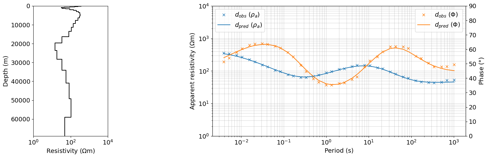
Run Sparse norm inverion with p_s=2 and p_z=0
recovered_model_ps_2_pz_0, output_dict_ps_2_pz_0 = run_fixed_layer_inversion(
    dobs,
    standard_deviation,
    rho_0,
    rho_ref,
    maxIter=40,
    maxIterCG=30,
    alpha_s=1e-10,
    alpha_z=1,
    beta0_ratio=1,
    coolingFactor=2,
    coolingRate=1,
    chi_factor=1,
    use_irls=True,
    p_s=2,
    p_z=0
)
1e-10 2500.0
Running inversion with SimPEG v0.22.2
simpeg.InvProblem is setting bfgsH0 to the inverse of the eval2Deriv.
***Done using same Solver, and solver_opts as the Simulation1DRecursive problem***
model has any nan: 0
============================ Inexact Gauss Newton ============================
# beta phi_d phi_m f |proj(x-g)-x| LS Comment
-----------------------------------------------------------------------------
x0 has any nan: 0
0 1.64e+04 6.78e+03 0.00e+00 6.78e+03 3.96e+03 0
1 8.19e+03 5.51e+02 1.16e-02 6.46e+02 8.47e+02 0
2 4.09e+03 7.91e+01 1.27e-02 1.31e+02 2.26e+02 0
Reached starting chifact with l2-norm regularization: Start IRLS steps...
irls_threshold 1.8081260512062256
3 2.05e+03 3.65e+01 2.16e-03 4.09e+01 5.46e+01 0
4 4.32e+03 3.33e+01 7.14e-03 6.42e+01 1.04e+02 0 Skip BFGS
5 9.57e+03 3.05e+01 7.78e-03 1.05e+02 8.49e+01 1
6 1.87e+04 3.87e+01 7.06e-03 1.71e+02 8.47e+01 0
7 3.45e+04 4.40e+01 8.70e-03 3.44e+02 1.26e+02 0
8 3.45e+04 8.06e+01 9.06e-03 3.93e+02 6.34e+01 0
9 2.61e+04 9.66e+01 1.15e-02 3.98e+02 2.97e+01 0 Skip BFGS
10 1.97e+04 9.77e+01 1.51e-02 3.95e+02 6.06e+01 0
11 1.51e+04 9.47e+01 1.92e-02 3.84e+02 1.05e+02 0
12 1.19e+04 8.89e+01 2.48e-02 3.84e+02 1.50e+02 0
13 9.41e+03 8.95e+01 3.44e-02 4.14e+02 1.92e+02 0
14 6.69e+03 1.10e+02 4.68e-02 4.23e+02 2.83e+02 0
15 4.37e+03 1.33e+02 5.22e-02 3.61e+02 1.71e+02 0
16 2.99e+03 1.20e+02 5.76e-02 2.92e+02 1.04e+02 0
17 2.21e+03 1.02e+02 5.84e-02 2.31e+02 8.26e+01 0
18 1.76e+03 8.77e+01 5.57e-02 1.86e+02 1.13e+02 0 Skip BFGS
19 1.76e+03 8.08e+01 4.92e-02 1.67e+02 6.94e+01 0 Skip BFGS
20 1.76e+03 7.81e+01 3.83e-02 1.45e+02 1.10e+02 0
21 1.76e+03 7.41e+01 2.82e-02 1.24e+02 1.10e+02 0
22 1.76e+03 6.67e+01 2.15e-02 1.05e+02 1.09e+02 0
23 2.81e+03 6.20e+01 1.53e-02 1.05e+02 8.13e+01 0 Skip BFGS
24 2.81e+03 6.85e+01 1.00e-02 9.66e+01 6.87e+01 0
25 2.81e+03 6.74e+01 6.00e-03 8.43e+01 8.22e+01 0
26 4.50e+03 6.13e+01 3.52e-03 7.72e+01 1.73e+02 0
27 7.33e+03 5.89e+01 1.44e-03 6.94e+01 2.32e+02 0
28 1.19e+04 5.96e+01 8.76e-04 7.00e+01 8.20e+01 0 Skip BFGS
29 1.92e+04 6.00e+01 5.74e-04 7.10e+01 7.44e+01 0
30 3.08e+04 6.15e+01 3.81e-04 7.32e+01 1.85e+02 0
31 4.90e+04 6.24e+01 2.50e-04 7.46e+01 9.97e+02 0
32 7.80e+04 6.27e+01 1.35e-04 7.32e+01 1.30e+03 0
33 1.24e+05 6.27e+01 8.98e-05 7.39e+01 2.33e+02 0
34 1.97e+05 6.27e+01 6.15e-05 7.49e+01 9.28e+01 0
35 3.13e+05 6.31e+01 4.28e-05 7.65e+01 8.27e+01 0
36 4.96e+05 6.31e+01 3.03e-05 7.81e+01 9.19e+01 0
37 7.87e+05 6.31e+01 2.19e-05 8.04e+01 8.79e+01 0
38 1.25e+06 6.31e+01 1.64e-05 8.36e+01 8.60e+01 0
39 1.98e+06 6.34e+01 1.27e-05 8.85e+01 8.68e+01 0
40 3.13e+06 6.34e+01 1.02e-05 9.55e+01 9.67e+01 0
------------------------- STOP! -------------------------
1 : |fc-fOld| = 6.9449e+00 <= tolF*(1+|f0|) = 6.7843e+02
1 : |xc-x_last| = 1.1409e-05 <= tolX*(1+|x0|) = 2.6641e+00
0 : |proj(x-g)-x| = 9.6697e+01 <= tolG = 1.0000e-40
0 : |proj(x-g)-x| = 9.6697e+01 <= 1e3*eps = 1.0000e-27
1 : maxIter = 40 <= iter = 40
------------------------- DONE! -------------------------
iteration = 40
dpred = output_dict_ps_2_pz_0[iteration]['dpred']
m = output_dict_ps_2_pz_0[iteration]['m']
fig = plt.figure(figsize=(16, 5))
gs = gridspec.GridSpec(1, 5, figure=fig)

ax0 = fig.add_subplot(gs[0, 0])
plot_1d_layer_model(
    layer_thicknesses_inv[::-1],
    (1./(np.exp(m)))[::-1],
    ax=ax0,
    color="k",**{'linestyle':'-'},
)
# ax0.legend()
ax0.set_xlabel(r"Resistivity ($\Omega$m)")
# ax0.set_xlim(1, 1e4)

ax = fig.add_subplot(gs[0, 2:])
ax.loglog(1./frequencies, dobs.reshape((len(frequencies), 2))[:,0], 'x', color='C0', label=r'$d_{obs}$ ($\rho_{a}$)')
ax.loglog(1./frequencies, dpred.reshape((len(frequencies), 2))[:,0], color='C0', label=r'$d_{pred}$ ($\rho_{a}$)')

ax_1 = ax.twinx()
ax_1.plot(1./frequencies, dobs.reshape((len(frequencies), 2))[:,1], 'x', color='C1', label=r'$d_{obs}$ ($\Phi$)')
ax_1.plot(1./frequencies, dpred.reshape((len(frequencies), 2))[:,1], color='C1', label=r'$d_{pred}$ ($\Phi$)')
ax.set_xlabel("Period (s)")
ax.grid(True, which='both', alpha=0.5)
ax.set_ylabel(r"Apparent resistivity ($\Omega$m)")
ax_1.set_ylabel(r"Phase ($\degree$)")
# ax.legend(bbox_to_anchor=(1.1,1))
ax.legend(loc=2)
ax_1.legend(loc=1)
ax.set_ylim(1, 10000)
ax_1.set_ylim(0, 90)
ax0.set_xlim(1, 10000)
plt.show()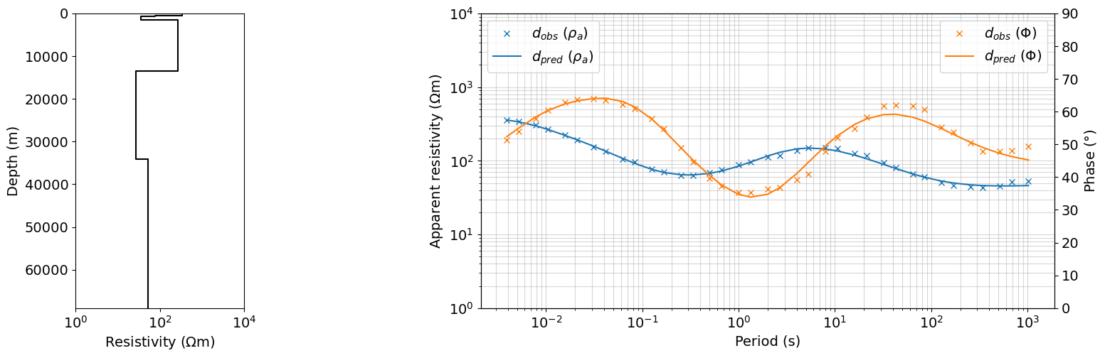
Run sparse norm inverion with p_s=0 and p_z=0
recovered_model_ps_0_pz_0, output_dict_ps_0_pz_0 = run_fixed_layer_inversion(
    dobs,
    standard_deviation,
    rho_0,
    rho_ref,
    maxIter=40,
    maxIterCG=30,
    alpha_s=1,
    alpha_z=1,
    beta0_ratio=1,
    coolingFactor=2,
    coolingRate=1,
    chi_factor=1,
    use_irls=True,
    p_s=0,
    p_z=0
)
1.0 2500.0
Running inversion with SimPEG v0.22.2
simpeg.InvProblem is setting bfgsH0 to the inverse of the eval2Deriv.
***Done using same Solver, and solver_opts as the Simulation1DRecursive problem***
model has any nan: 0
============================ Inexact Gauss Newton ============================
# beta phi_d phi_m f |proj(x-g)-x| LS Comment
-----------------------------------------------------------------------------
x0 has any nan: 0
0 1.07e-01 6.78e+03 0.00e+00 6.78e+03 3.96e+03 0
1 5.35e-02 1.92e+03 9.80e+03 2.45e+03 1.06e+03 0
2 2.68e-02 7.71e+02 1.70e+04 1.23e+03 4.59e+02 0
3 1.34e-02 2.90e+02 2.56e+04 6.33e+02 2.44e+02 0 Skip BFGS
4 6.69e-03 1.17e+02 3.28e+04 3.36e+02 1.10e+02 0 Skip BFGS
Reached starting chifact with l2-norm regularization: Start IRLS steps...
irls_threshold 1.8216907667058009
5 3.35e-03 5.62e+01 5.47e+04 2.39e+02 5.88e+01 0 Skip BFGS
6 5.44e-03 5.91e+01 5.72e+04 3.70e+02 3.25e+02 0
7 4.34e-03 8.75e+01 3.54e+04 2.41e+02 1.50e+02 0
8 3.31e-03 9.55e+01 2.51e+04 1.79e+02 1.09e+02 0 Skip BFGS
9 2.56e-03 9.29e+01 1.70e+04 1.36e+02 2.45e+01 0 Skip BFGS
10 2.02e-03 8.93e+01 1.33e+04 1.16e+02 4.15e+01 0 Skip BFGS
11 1.63e-03 8.55e+01 1.05e+04 1.03e+02 3.26e+01 0 Skip BFGS
12 1.63e-03 8.08e+01 8.20e+03 9.41e+01 5.21e+01 0 Skip BFGS
13 1.63e-03 7.06e+01 5.81e+03 8.01e+01 6.96e+01 0
14 2.80e-03 5.14e+01 3.68e+03 6.18e+01 5.86e+01 0
15 5.23e-03 4.28e+01 2.26e+03 5.47e+01 5.04e+01 0 Skip BFGS
16 9.86e-03 4.18e+01 1.41e+03 5.57e+01 4.86e+01 0 Skip BFGS
17 1.85e-02 4.21e+01 9.33e+02 5.94e+01 5.04e+01 0
18 3.45e-02 4.28e+01 6.21e+02 6.42e+01 5.16e+01 0
19 6.36e-02 4.40e+01 4.13e+02 7.02e+01 4.61e+01 0
20 1.15e-01 4.58e+01 2.75e+02 7.75e+01 5.22e+01 0
21 2.02e-01 4.87e+01 1.84e+02 8.58e+01 6.57e+01 0
22 3.44e-01 5.28e+01 1.22e+02 9.49e+01 7.98e+01 0
23 5.61e-01 5.87e+01 8.15e+01 1.04e+02 8.44e+01 0
24 8.73e-01 6.66e+01 5.44e+01 1.14e+02 9.81e+01 0
25 8.73e-01 7.65e+01 3.63e+01 1.08e+02 4.96e+01 0
26 8.73e-01 8.10e+01 2.42e+01 1.02e+02 2.57e+01 0 Skip BFGS
27 8.73e-01 8.13e+01 1.62e+01 9.54e+01 3.72e+01 0 Skip BFGS
28 8.73e-01 7.55e+01 1.08e+01 8.49e+01 6.43e+01 0
29 1.42e+00 5.92e+01 7.18e+00 6.94e+01 8.04e+01 0
30 2.55e+00 4.63e+01 4.78e+00 5.85e+01 6.54e+01 0 Skip BFGS
31 4.76e+00 4.28e+01 3.19e+00 5.80e+01 4.42e+01 0 Skip BFGS
32 8.88e+00 4.26e+01 2.12e+00 6.15e+01 4.71e+01 0 Skip BFGS
33 1.65e+01 4.33e+01 1.42e+00 6.66e+01 5.90e+01 0
34 3.01e+01 4.46e+01 1.05e+00 7.62e+01 7.62e+01 0
35 5.36e+01 4.76e+01 7.06e-01 8.55e+01 5.38e+02 0
36 9.17e+01 5.20e+01 4.68e-01 9.49e+01 1.79e+04 0
37 1.50e+02 5.80e+01 3.06e-01 1.04e+02 6.69e+04 0
38 2.34e+02 6.59e+01 2.00e-01 1.13e+02 2.92e+03 0
39 2.34e+02 7.58e+01 1.33e-01 1.07e+02 4.20e+02 0
40 2.34e+02 8.09e+01 8.94e-02 1.02e+02 6.73e+01 0 Skip BFGS
------------------------- STOP! -------------------------
1 : |fc-fOld| = 5.1560e+00 <= tolF*(1+|f0|) = 6.7843e+02
1 : |xc-x_last| = 1.3693e-01 <= tolX*(1+|x0|) = 2.6641e+00
0 : |proj(x-g)-x| = 6.7259e+01 <= tolG = 1.0000e-40
0 : |proj(x-g)-x| = 6.7259e+01 <= 1e3*eps = 1.0000e-27
1 : maxIter = 40 <= iter = 40
------------------------- DONE! -------------------------
iteration = 40
dpred = output_dict_ps_0_pz_0[iteration]['dpred']
m = output_dict_ps_0_pz_0[iteration]['m']
fig = plt.figure(figsize=(16, 5))
gs = gridspec.GridSpec(1, 5, figure=fig)

ax0 = fig.add_subplot(gs[0, 0])
plot_1d_layer_model(
    layer_thicknesses_inv[::-1],
    (1./(np.exp(m)))[::-1],
    ax=ax0,
    color="k",**{'linestyle':'-'},
)
# ax0.legend()
ax0.set_xlabel(r"Resistivity ($\Omega$m)")
# ax0.set_xlim(1, 1e4)

ax = fig.add_subplot(gs[0, 2:])
ax.loglog(1./frequencies, dobs.reshape((len(frequencies), 2))[:,0], 'x', color='C0', label=r'$d_{obs}$ ($\rho_{a}$)')
ax.loglog(1./frequencies, dpred.reshape((len(frequencies), 2))[:,0], color='C0', label=r'$d_{pred}$ ($\rho_{a}$)')

ax_1 = ax.twinx()
ax_1.plot(1./frequencies, dobs.reshape((len(frequencies), 2))[:,1], 'x', color='C1', label=r'$d_{obs}$ ($\Phi$)')
ax_1.plot(1./frequencies, dpred.reshape((len(frequencies), 2))[:,1], color='C1', label=r'$d_{pred}$ ($\Phi$)')
ax.set_xlabel("Period (s)")
ax.grid(True, which='both', alpha=0.5)
ax.set_ylabel(r"Apparent resistivity ($\Omega$m)")
ax_1.set_ylabel(r"Phase ($\degree$)")
# ax.legend(bbox_to_anchor=(1.1,1))
ax.legend(loc=2)
ax_1.legend(loc=1)
ax.set_ylim(1, 10000)
ax_1.set_ylim(0, 90)
ax0.set_xlim(1, 10000)
plt.show()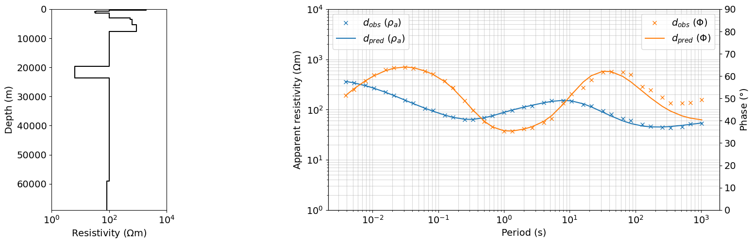
matplotlib.rcParams['font.size'] = 12
fig, axs = plt.subplots(1,3, figsize=(12, 8))
ax1, ax2, ax3 = axs
plot_1d_layer_model(
    layer_thicknesses_inv[::-1],
    (1./(np.exp(recovered_model)))[::-1],
    ax=ax1,
    color="k",**{'linestyle':'-'},
)
ax1.plot(rho_ref*np.ones([2,]), np.array([0, 70000]), color="b",**{'linestyle':'--'})

plot_1d_layer_model(
    layer_thicknesses_inv[::-1],
    (1./(np.exp(recovered_model_ps_2_pz_0)))[::-1],
    ax=ax2,
    color="k",**{'linestyle':'-'},
)
ax2.plot(rho_ref*np.ones([2,]), np.array([0, 70000]), color="b",**{'linestyle':'--'})

plot_1d_layer_model(
    layer_thicknesses_inv[::-1],
    (1./(np.exp(recovered_model_ps_0_pz_0)))[::-1],
    ax=ax3,
    color="k",**{'linestyle':'-'},
)
ax3.plot(rho_ref*np.ones([2,]), np.array([0, 70000]), color="b",**{'linestyle':'--'})

titles = [r"Smooth ($p_{s}=2, p_{z}=2$)", "Sharp ($p_{s}=2, p_{z}=0$)", "Compact + Sharp ($p_{s}=0, p_{z}=0$)"]
for ii, ax in enumerate(axs):
    ax.set_xlabel("Resistivity ($\Omega$m)")
    if ii>0:
        ax.set_yticklabels([])
        ax.set_ylabel("")
    ax.set_title(titles[ii])
    ax.set_xlim(1, 1000)
plt.tight_layout()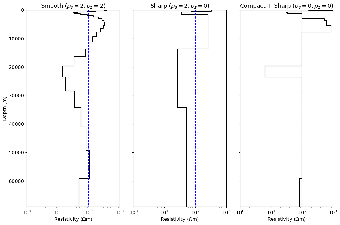
# Experimental plotting code for MTpy# mesh_inv = TensorMesh([(np.r_[layer_thicknesses_inv, layer_thicknesses_inv[-1]])], "N")
# receivers_list = [
# nsem.receivers.PointNaturalSource(component="real"),
# nsem.receivers.PointNaturalSource(component="imag"),
# ]
# source_list = []
# for freq in frequencies:
# source_list.append(nsem.sources.Planewave(receivers_list, freq))
# survey = nsem.survey.Survey(source_list)
# sigma_map = maps.ExpMap(nP=len(layer_thicknesses_inv)+1)
# simulation = nsem.simulation_1d.Simulation1DRecursive(
# survey=survey,
# sigmaMap=sigma_map,
# thicknesses=layer_thicknesses_inv,
# )# dobs = np.c_[tf.Z.res_xy, tf.Z.phase_xy].flatten()# tf.Z.z[:,]# dpred = simulation.dpred(m)# plt.plot(dpred)## Plot using `MTpy`?# from mtpy import MT
# from mtpy.core import Z
# n_freq = len(frequencies)
# app_rho_matrix = np.zeros((n_freq, 2, 2), dtype=float)
# phase_matrix = np.zeros((n_freq, 2, 2), dtype=float)
# app_rho_matrix[:,0,1] = dpred.reshape((len(frequencies), 2))[:,0]
# app_rho_matrix[:,1,0] = dpred.reshape((len(frequencies), 2))[:,0]
# phase_matrix[:,0,1] = dpred.reshape((len(frequencies), 2))[:,1]
# phase_matrix[:,1,0] = dpred.reshape((len(frequencies), 2))[:,1]-180
# # or add apparent resistivity and phase
# z_object = Z()
# z_object.set_resistivity_phase(app_rho_matrix, phase_matrix, frequencies)
# tf_pred = MT()
# tf_pred.Z = z_object
# tf_pred.survey_metadata.id = tf.survey_metadata.id
# tf_pred.station_metadata.id = 'ynp05s_pred'
# tf_pred.station_metadata.transfer_function.id = 'ynp05s_pred'
# # if this is 2D maybe we need a location
# tf_pred.station_metadata.location.latitude = tf.station_metadata.location.latitude
# tf_pred.station_metadata.location.longitude = tf.station_metadata.location.longitude
# # mc.add_tf(tf_pred)# mc.plot_mt_response(['YNP05S', 'ynp05s_pred'], plot_style="compare", plot_tipper='n')