Learning goals
Understand the concept of Tikhonov curve - impact of the trade-off parameter
betaUnderstand the concept of overfitting and underfitting
Understand of the concept of depth-of-investigation (DOI)
import numpy as np
from simpeg.electromagnetics import natural_source as nsem
from simpeg import maps
import matplotlib.pyplot as plt
import matplotlib
import matplotlib.gridspec as gridspec
from simpeg.utils import plot_1d_layer_model
from discretize import TensorMesh
from simpeg import (
    maps,
    data,
    data_misfit,
    regularization,
    optimization,
    inverse_problem,
    inversion,
    directives,
    utils,
)
matplotlib.rcParams['font.size'] = 14
Generate synthetic MT data
def run_forward(layer_thicknesses, rho_layers, frequencies, relative_error_rho=0.05, floor_phase=2):
    mesh = TensorMesh([(np.r_[layer_thicknesses, layer_thicknesses[-1]])], "N")

    wire_map = maps.Wires(("sigma", mesh.nC), ("t", mesh.nC - 1))
    sigma_map = maps.ExpMap(nP=mesh.nC) * wire_map.sigma
    layer_map = maps.ExpMap(nP=mesh.nC - 1) * wire_map.t


    sigma_map = maps.ExpMap(nP=len(rho_layers))

    receivers_list = [
        nsem.receivers.PointNaturalSource(component="app_res"),
        nsem.receivers.PointNaturalSource(component="phase"),
    ]

    source_list = []
    for freq in frequencies:
        source_list.append(nsem.sources.Planewave(receivers_list, freq))

    survey = nsem.survey.Survey(source_list)

    simulation = nsem.simulation_1d.Simulation1DRecursive(
        survey=survey,
        sigmaMap=sigma_map,
        thicknesses=layer_thicknesses,
    )

    true_model = np.r_[np.log(1./rho_layers)]

    dpred = simulation.dpred(true_model)
    rho_app = dpred.reshape((len(frequencies), 2))[:,0]
    phase = dpred.reshape((len(frequencies), 2))[:,1]
    std = np.c_[abs(rho_app)*relative_error_rho, np.ones(len(phase))*floor_phase].flatten()
    noise = np.c_[np.random.randn(rho_app.size)*relative_error_rho*abs(rho_app), np.random.randn(rho_app.size)*floor_phase].flatten()
    dobs = dpred + noise
    return dobs
layer_tops = np.r_[0., -600., -1991., -5786., -9786.][::-1] # in m
layer_thicknesses = np.diff(layer_tops)
rho_layers = np.r_[250., 25, 100., 10., 25.][::-1]
# frequencies = np.logspace(0, 3, 31)
frequencies = np.logspace(-3, 3, 31)
relative_error_rho = 0.05
floor_phase = 2.
dobs = run_forward(layer_thicknesses, rho_layers, frequencies, relative_error_rho=relative_error_rho, floor_phase=floor_phase)fig = plt.figure(figsize=(16, 5))
gs = gridspec.GridSpec(1, 5, figure=fig)
ax0 = fig.add_subplot(gs[0, 0])
plot_1d_layer_model(layer_thicknesses[::-1], rho_layers[::-1], ax=ax0, color="k", **{'label':'True'})
ax0.set_xlabel(r"Resistivity [$\Omega$m]")
ax0.set_xlim(1, 1000)
# ax0.set_yscale('log')
ax = fig.add_subplot(gs[0, 2:])
ax.loglog(frequencies, dobs.reshape((len(frequencies), 2))[:,0], color='C0', label=r'$\rho_{a}$')
ax.loglog(frequencies[0], dobs.reshape((len(frequencies), 2))[0,0], color='C1', label=r'$\Phi$')
ax_1 = ax.twinx()
ax_1.plot(frequencies, dobs.reshape((len(frequencies), 2))[:,1], color='C1')
ax.set_xlabel("Frequency (Hz)")
ax.set_ylim(10, 1000)
ax_1.set_ylim(0, 90)
ax.grid(True, which='both', alpha=0.5)
ax.set_ylabel(r"Apparent resistivity ($\rho_{a}$) [$\Omega$m]")
ax_1.set_ylabel(r"Phase ($\Phi$) [$\degree$]")
ax.legend(bbox_to_anchor=(-0.1, 1))
ax.set_xlim(frequencies.max(), frequencies.min())
plt.show()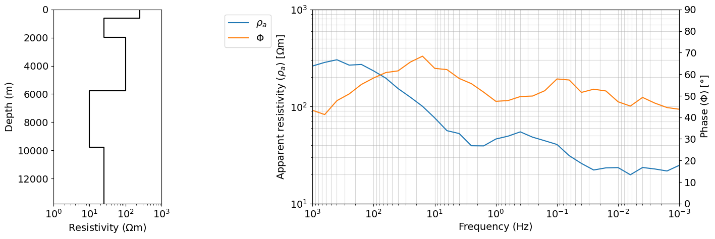
Run MT inversion
dz = 10
n_layer = 35
z_factor = 1.18
layer_thicknesses_inv = dz*z_factor**np.arange(n_layer-1)[::-1]
layer_thicknesses_inv.sum() / 1e315.386878068914159def run_smooth_inversion(
dobs,
standard_deviation,
rho_0,
rho_ref,
maxIter=10,
maxIterCG=30,
maxIterLS=30,
alpha_s=1e-10,
alpha_z=1,
beta0_ratio=1,
coolingFactor=2,
coolingRate=1,
chi_factor=1,
p_s=0,
p_z=0,
):
mesh_inv = TensorMesh([(np.r_[layer_thicknesses_inv, layer_thicknesses_inv[-1]])], "N")
receivers_list = [
nsem.receivers.PointNaturalSource(component="app_res"),
nsem.receivers.PointNaturalSource(component="phase"),
]
source_list = []
for freq in frequencies:
source_list.append(nsem.sources.Planewave(receivers_list, freq))
survey = nsem.survey.Survey(source_list)
sigma_map = maps.ExpMap(nP=len(layer_thicknesses_inv)+1)
simulation = nsem.simulation_1d.Simulation1DRecursive(
survey=survey,
sigmaMap=sigma_map,
thicknesses=layer_thicknesses_inv,
)
# Define the data
data_object = data.Data(survey, dobs=dobs, standard_deviation=standard_deviation)
# Initial model
m0 = np.ones(len(layer_thicknesses_inv)+1) * np.log(1./rho_0)
# Reference model
mref = np.ones(len(layer_thicknesses_inv)+1) * np.log(1./rho_ref)
dmis = data_misfit.L2DataMisfit(simulation=simulation, data=data_object)
# Define the regularization (model objective function)
reg = regularization.Sparse(
mesh_inv, alpha_s=alpha_s, alpha_x=alpha_z,
reference_model=mref,
reference_model_in_smooth=False,
mapping=maps.IdentityMap(mesh=mesh_inv),
# norms=[p_s, p_z]
)
# reg.gradient_type = 'components'
# Define how the optimization problem is solved. Here we will use an inexact
# Gauss-Newton approach that employs the conjugate gradient solver.
opt = optimization.InexactGaussNewton(maxIter=maxIter, maxIterCG=maxIterCG, maxIterLS=maxIterLS)
# Define the inverse problem
inv_prob = inverse_problem.BaseInvProblem(dmis, reg, opt)
#######################################################################
# Define Inversion Directives
# ---------------------------
#
# Here we define any directives that are carried out during the inversion. This
# includes the cooling schedule for the trade-off parameter (beta), stopping
# criteria for the inversion and saving inversion results at each iteration.
#
# Defining a starting value for the trade-off parameter (beta) between the data
# misfit and the regularization.
starting_beta = directives.BetaEstimate_ByEig(beta0_ratio=beta0_ratio)
# Set the rate of reduction in trade-off parameter (beta) each time the
# the inverse problem is solved. And set the number of Gauss-Newton iterations
# for each trade-off paramter value.
beta_schedule = directives.BetaSchedule(coolingFactor=coolingFactor, coolingRate=coolingRate)
save_dictionary = directives.SaveOutputDictEveryIteration()
save_dictionary.outDict = {}
# Setting a stopping criteria for the inversion.
target_misfit = directives.TargetMisfit(chifact=chi_factor)
precond = directives.UpdatePreconditioner()
# The directives are defined as a list.
directives_list = [
precond,
starting_beta,
beta_schedule,
target_misfit,
save_dictionary
]
#####################################################################
# Running the Inversion
# ---------------------
#
# To define the inversion object, we need to define the inversion problem and
# the set of directives. We can then run the inversion.
#
# Here we combine the inverse problem and the set of directives
inv = inversion.BaseInversion(inv_prob, directives_list)
# Run the inversion
recovered_model = inv.run(m0)
return recovered_model, save_dictionary.outDictrho_app = dobs.reshape((len(frequencies), 2))[:,0]
phase = dobs.reshape((len(frequencies), 2))[:,1]
standard_deviation = np.c_[abs(rho_app)*relative_error_rho, np.ones(len(phase))*floor_phase].flatten()
rho_0 = 20
rho_ref = 100.
output_dict ={}
recovered_model, output_dict = run_smooth_inversion(
dobs,
standard_deviation,
rho_0,
rho_ref,
maxIter=30,
maxIterCG=30,
maxIterLS=50,
alpha_s=1e-5,
alpha_z=1,
beta0_ratio=1e2,
coolingFactor=2,
coolingRate=1,
chi_factor=1e-2
)
Running inversion with SimPEG v0.22.2

                        simpeg.InvProblem is setting bfgsH0 to the inverse of the eval2Deriv.
                        ***Done using same Solver, and solver_opts as the Simulation1DRecursive problem***

model has any nan: 0
============================ Inexact Gauss Newton ============================
  #     beta     phi_d     phi_m       f      |proj(x-g)-x|  LS    Comment
-----------------------------------------------------------------------------
x0 has any nan: 0
   0  1.29e+05  5.72e+03  3.99e-01  5.70e+04    1.85e+04      0
   1  6.43e+04  2.89e+04  8.01e-03  2.94e+04    3.05e+04      0
   2  3.21e+04  6.98e+03  7.73e-02  9.47e+03    3.51e+03      0
   3  1.61e+04  1.92e+03  1.38e-01  4.13e+03    7.28e+02      0   Skip BFGS
   4  8.04e+03  1.20e+03  1.68e-01  2.54e+03    6.06e+02      0   Skip BFGS
   5  4.02e+03  6.05e+02  2.14e-01  1.47e+03    3.31e+02      0
   6  2.01e+03  2.69e+02  2.59e-01  7.89e+02    1.64e+02      0
   7  1.00e+03  1.38e+02  2.85e-01  4.25e+02    4.53e+01      0
   8  5.02e+02  1.01e+02  2.97e-01  2.50e+02    1.06e+02      0
   9  2.51e+02  9.09e+01  2.92e-01  1.64e+02    1.37e+02      1
  10  1.26e+02  8.90e+01  2.90e-01  1.25e+02    2.30e+02      0   Skip BFGS
  11  6.28e+01  7.10e+01  2.83e-01  8.88e+01    3.21e+01      0   Skip BFGS
  12  3.14e+01  6.35e+01  3.51e-01  7.46e+01    1.13e+02      0   Skip BFGS
  13  1.57e+01  5.85e+01  3.55e-01  6.40e+01    1.61e+01      0
  14  7.85e+00  5.78e+01  3.60e-01  6.07e+01    3.85e+01      1   Skip BFGS
  15  3.92e+00  5.73e+01  3.55e-01  5.87e+01    3.57e+00      0
  16  1.96e+00  5.72e+01  3.64e-01  5.80e+01    3.92e+01      2   Skip BFGS
  17  9.81e-01  5.67e+01  3.58e-01  5.70e+01    2.98e+00      0
  18  4.91e-01  5.65e+01  3.70e-01  5.67e+01    1.47e+01      4   Skip BFGS
  19  2.45e-01  5.64e+01  3.96e-01  5.65e+01    2.91e+01      3
  20  1.23e-01  5.61e+01  3.99e-01  5.61e+01    2.32e+00      0
  21  6.13e-02  5.59e+01  4.15e-01  5.60e+01    8.18e+00      6   Skip BFGS
  22  3.07e-02  5.59e+01  4.46e-01  5.59e+01    1.30e+01      6
  23  1.53e-02  5.58e+01  5.08e-01  5.58e+01    1.69e+01      5   Skip BFGS
  24  7.66e-03  5.58e+01  6.54e-01  5.58e+01    2.09e+01      5   Skip BFGS
  25  3.83e-03  5.56e+01  8.52e-01  5.56e+01    2.33e+00      0   Skip BFGS
  26  1.92e-03  5.56e+01  8.99e-01  5.56e+01    1.06e+01      7   Skip BFGS
  27  9.58e-04  5.56e+01  9.29e-01  5.56e+01    1.35e+01      7   Skip BFGS
  28  4.79e-04  5.55e+01  1.24e+00  5.55e+01    1.48e+01      6   Skip BFGS
  29  2.40e-04  5.55e+01  1.27e+00  5.55e+01    1.68e+01      6   Skip BFGS
  30  1.20e-04  5.55e+01  3.64e+00  5.55e+01    1.81e+01      4   Skip BFGS
------------------------- STOP! -------------------------
1 : |fc-fOld| = 5.7294e-03 <= tolF*(1+|f0|) = 5.7003e+03
0 : |xc-x_last| = 6.5772e+00 <= tolX*(1+|x0|) = 1.8723e+00
0 : |proj(x-g)-x|    = 1.8125e+01 <= tolG          = 1.0000e-01
0 : |proj(x-g)-x|    = 1.8125e+01 <= 1e3*eps       = 1.0000e-02
1 : maxIter   =      30    <= iter          =     30
------------------------- DONE! -------------------------
target_misfit = dobs.size
iterations = list(output_dict.keys())
n_iteration = len(iterations)
phi_ds = np.zeros(n_iteration)
phi_ms = np.zeros(n_iteration)
betas = np.zeros(n_iteration)
for ii, iteration in enumerate(iterations):
    phi_ds[ii] = output_dict[iteration]['phi_d']
    phi_ms[ii] = output_dict[iteration]['phi_m']
    betas[ii] = output_dict[iteration]['beta']
matplotlib.rcParams['font.size'] = 14
def tikhonov_curve(iteration, scale='log'):
fig, ax = plt.subplots(1,1, figsize=(5,5))
ax.plot(phi_ms, phi_ds)
ax.plot(phi_ms[iteration-1], phi_ds[iteration-1], 'ro')
ax.set_xlabel(r"$\phi_m$")
ax.set_ylabel(r"$\phi_d$")
if scale == 'log':
ax.set_xscale('log')
ax.set_yscale('log')
xlim = ax.get_xlim()
ax.plot(xlim, np.ones(2) * target_misfit, '--')
ax.set_title("Iteration={:d}, Beta = {:.1e}".format(iteration, betas[iteration-1]))
ax.set_xlim(xlim)
plt.show()from ipywidgets import interact, widgets
Q_iter = interact(
tikhonov_curve,
iteration=widgets.IntSlider(min=1, max=int(n_iteration), value=n_iteration),
scale=widgets.RadioButtons(options=['linear', 'log'])
)Loading...
iteration = Q_iter.widget.kwargs['iteration']
dpred = output_dict[iteration]['dpred']
m = output_dict[iteration]['m']
fig = plt.figure(figsize=(16, 5))
gs = gridspec.GridSpec(1, 5, figure=fig)

ax0 = fig.add_subplot(gs[0, 0])
plot_1d_layer_model(layer_thicknesses[::-1], rho_layers[::-1], ax=ax0, color="k", **{'label':r'$m_{True}$'})
plot_1d_layer_model(
    layer_thicknesses_inv[::-1],
    (1./(np.exp(m)))[::-1],
    ax=ax0,
    color="k",**{'label':r'$m_{Inv}$', 'linestyle':'--'}
)
ax0.legend()
ax0.set_xlabel(r"Resistivity [$\Omega$m]")
ax0.set_xlim(1, 1e4)
ax0.set_title('Model from iteration ' + str(iteration), fontsize=14)

ax = fig.add_subplot(gs[0, 2:])
ax.loglog(1./frequencies, dobs.reshape((len(frequencies), 2))[:,0], 'x', color='C0', label=r'$d_{obs}$ ($\rho_{a}$)')
ax.loglog(1./frequencies, dpred.reshape((len(frequencies), 2))[:,0], color='C0', label=r'$d_{pred}$ ($\rho_{a}$)')

ax_1 = ax.twinx()
ax_1.plot(1./frequencies, dobs.reshape((len(frequencies), 2))[:,1], 'x', color='C1', label=r'$d_{obs}$ ($\Phi$)')
ax_1.plot(1./frequencies, dpred.reshape((len(frequencies), 2))[:,1], color='C1', label=r'$d_{pred}$ ($\Phi$)')
ax.set_xlabel("Period [s]")
ax.grid(True, which='both', alpha=0.5)
ax.set_ylabel(r"Apparent resistivity [$\Omega$m]")
ax_1.set_ylabel(r"Phase [$\degree$]")
# ax.legend(bbox_to_anchor=(1.1,1))
ax.legend(loc=2)
ax_1.legend(loc=1)
ax.set_ylim(1, 10000)
ax_1.set_ylim(0, 90)
ax0.set_xlim(1, 10000)
plt.show()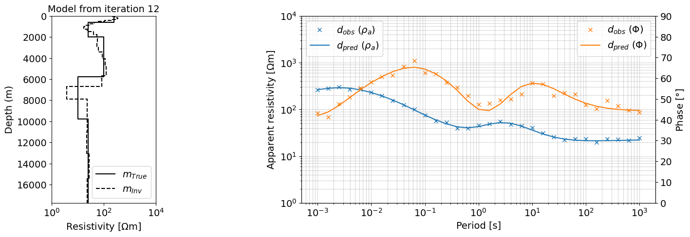
use_doi_index = False
if use_doi_index:
    rho_ref_1 = 50
    m1, _ = run_smooth_inversion(
        dobs,
        standard_deviation,
        rho_0,
        rho_ref_1,
        maxIter=10,
        maxIterCG=30,
        alpha_s=0.1,
        alpha_z=1,
        beta0_ratio=1e1,
        coolingFactor=2,
        coolingRate=1,
        chi_factor=1
    )

    rho_ref_2 = 100
    m2, _ = run_smooth_inversion(
        dobs,
        standard_deviation,
        rho_0,
        rho_ref_2,
        maxIter=10,
        maxIterCG=30,
        alpha_s=0.1,
        alpha_z=1,
        beta0_ratio=1e1,
        coolingFactor=2,
        coolingRate=1,
        chi_factor=1
    )

    def calculate_doi_index(m1, m2, mref1, mref2):
        doi_index = abs((m1-m2) / (mref1-mref2))
        doi_index /= doi_index.max()
        return doi_index

    mref1 = np.exp(1./rho_ref_1)
    mref2 = np.exp(1./rho_ref_2)
    doi_index = calculate_doi_index(m1, m2, mref1, mref2)

    fig, ax = plt.subplots(1,1, figsize=(3, 5))
    plot_1d_layer_model(
        layer_thicknesses_inv[::-1],
        (1./(np.exp(m)))[::-1],
        ax=ax,
        color="k",**{'label':'Pred', 'linestyle':'-'}
    )
    plot_1d_layer_model(
        layer_thicknesses_inv[::-1],
        (1./(np.exp(m1)))[::-1],
        ax=ax,
        color="C1",**{'label':'Pred', 'linestyle':'--'}
    )

    plot_1d_layer_model(
        layer_thicknesses_inv[::-1],
        (1./(np.exp(m2)))[::-1],
        ax=ax,
        color="C2",**{'label':'Pred', 'linestyle':'--'}
    )
    ax.set_xlim(1, 10000)
    ax_1 = ax.twiny()

    plot_1d_layer_model(
        layer_thicknesses_inv[::-1],
        doi_index[::-1],
        ax=ax_1,
        scale='linear',**{'label':'Pred', 'linestyle':'--'}
    )
    ax.set_xlabel(r"Resistivity ($\Omega$m)")
    ax_1.set_xlabel("DOI index")