Learning goals
Understand the sensitivity of apparent resistivity and phase with regard to layered structure
Understand the concept of an equivalent conductance
Conduct manual fitting of the field data
import numpy as np
from simpeg.electromagnetics import natural_source as nsem
from simpeg import maps
import matplotlib.pyplot as plt
import matplotlib
from simpeg.utils import plot_1d_layer_model
from discretize import TensorMesh
import warnings
warnings.filterwarnings("ignore")
Setup 1D MT simulation
frequencies = np.logspace(-5, 5, 101)
layer_thicknesses = np.array([1000, 1000])
rho = np.array([1000., 10, 1000.])
mesh = TensorMesh([(np.r_[layer_thicknesses, layer_thicknesses[-1]])], "0")

wire_map = maps.Wires(("sigma", mesh.nC), ("t", mesh.nC - 1))
sigma_map = maps.ExpMap(nP=mesh.nC) * wire_map.sigma
layer_map = maps.ExpMap(nP=mesh.nC - 1) * wire_map.t


model_mapping = maps.IdentityMap(nP=len(rho))

receivers_list = [
    nsem.receivers.PointNaturalSource(component="app_res"),
    nsem.receivers.PointNaturalSource(component="phase"),
]

source_list = []
for freq in frequencies:
    source_list.append(nsem.sources.Planewave(receivers_list, freq))

survey = nsem.survey.Survey(source_list)

simulation = nsem.simulation_1d.Simulation1DRecursive(
    survey=survey,
    sigmaMap=sigma_map,
    thicknessesMap=layer_map,
)

true_model = np.r_[np.log(1./rho), np.log(layer_thicknesses)]

dpred = simulation.dpred(true_model)
import matplotlib.gridspec as gridspec
def calculate_response(rho1, rho2, rho3, z, t):
model = np.log(np.r_[1./rho3, 1./rho2, 1./rho1, t, z])
pred = simulation.dpred(model)
# print (simulation.rho, simulation.thicknesses)
return pred
def plot_results(rho1, rho2, rho3, z, t, add_noise, rerr_amp, floor_phase, plot_option):
pred = calculate_response(rho1, rho2, rho3, z, t)
amp = pred.reshape((len(frequencies), 2))[:,0]
phase = pred.reshape((len(frequencies), 2))[:,1]
if add_noise:
noise = np.c_[np.random.randn(amp.size)*rerr_amp*abs(amp), np.random.randn(amp.size)*floor_phase].flatten()
pred += noise
fig = plt.figure(figsize=(16, 5))
gs = gridspec.GridSpec(1, 5, figure=fig)
ax0 = fig.add_subplot(gs[0, 0])
layer_thicknesses = np.array([z, t])
rho = np.r_[rho1, rho2, rho3]
plot_1d_layer_model(layer_thicknesses, rho, ax=ax0, color="k", **{'label':'True'})
ax0.set_xlabel("Resistivity ($\Omega$m)")
ax0.set_xlim(1, 10000)
ax = fig.add_subplot(gs[0, 2:])
if (plot_option == 'app_res') or (plot_option == 'both'):
ax.loglog(frequencies, pred.reshape((len(frequencies), 2))[:,0], color='C0', label='AppRes.', lw=3)
if (plot_option == 'phase') or (plot_option == 'both'):
ax.loglog(frequencies[0], pred.reshape((len(frequencies), 2))[0,0], color='C1', label='Phase')
ax_1 = ax.twinx()
ax_1.plot(frequencies, pred.reshape((len(frequencies), 2))[:,1], color='C1', lw=3)
ax_1.set_ylim(0, 90)
ax_1.set_ylabel("Phase ($\degree$)")
ax.set_xlabel("Frequency (Hz)")
ax.set_ylim(1, 10000)
ax.grid(True, which='both', alpha=0.5)
ax.set_ylabel("Apparent resistivity ($\Omega$m)")
ax.legend(bbox_to_anchor=(-0.1, 1))
ax.set_xlim(1e5, 1e-5)
plt.show()
# plt.tight_layout()Explore MT responses with variable 1D structure
from ipywidgets import widgets, interactQ = interact(
plot_results,
rho1=widgets.FloatLogSlider(base=10, value=100, min=0, max=4, continuous_update=True, description="$\\rho_1$"),
rho2=widgets.FloatLogSlider(base=10, value=5, min=0, max=4, continuous_update=True, description="$\\rho_2$"),
rho3=widgets.FloatLogSlider(base=10, value=100, min=0, max=4, continuous_update=True, description="$\\rho_3$"),
z=widgets.FloatLogSlider(base=10, value=3000, min=0, max=5, continuous_update=True, description="$z$"),
t=widgets.FloatLogSlider(base=10, value=1000, min=0, max=5, continuous_update=True, description="$thk$"),
add_noise=widgets.Checkbox(),
rerr_amp=widgets.FloatText(value=0.1),
floor_phase=widgets.FloatText(value=2),
plot_option=widgets.RadioButtons(options=['app_res', 'phase', 'both'])
)
QLoading...
Equivalent conductance
rho1 = 100.
rho3 = 100.
rho2 = 1.
z = 3000
t = 1000
# conductance
S = 1./rho2 * t
t_iter = np.arange(5) * 1000 + 1000

fig = plt.figure(figsize=(16*0.8, 5*0.8))
gs = gridspec.GridSpec(1, 5, figure=fig)
ax0 = fig.add_subplot(gs[0, 0])
ax = fig.add_subplot(gs[0, 2:])

for ii in range(len(t_iter)):
    rho2_iter = 1./(S/t_iter[ii])
    pred = calculate_response(rho1, rho2_iter, rho3, z, t_iter[ii])
    amp = pred.reshape((len(frequencies), 2))[:,0]
    phase = pred.reshape((len(frequencies), 2))[:,1]
    layer_thicknesses = np.array([z, t_iter[ii]])
    rho = np.r_[rho1, rho2_iter, rho3]
    plot_1d_layer_model(layer_thicknesses, rho, ax=ax0, color="k", **{'label':'True'})
    ax0.set_xlabel("Resistivity ($\Omega$m)")
    ax0.set_xlim(1, 10000)


    ax.loglog(frequencies, pred.reshape((len(frequencies), 2))[:,0], color='C0', lw=3)
    ax.set_xlabel("Frequency (Hz)")
    ax.set_ylim(1, 10000)
    ax.grid(True, which='both', alpha=0.5)
    ax.set_ylabel("Apparent resistivity ($\Omega$m)")
#     ax.legend(bbox_to_anchor=(-0.1, 1))
    ax.set_xlim(1e5, 1e-5)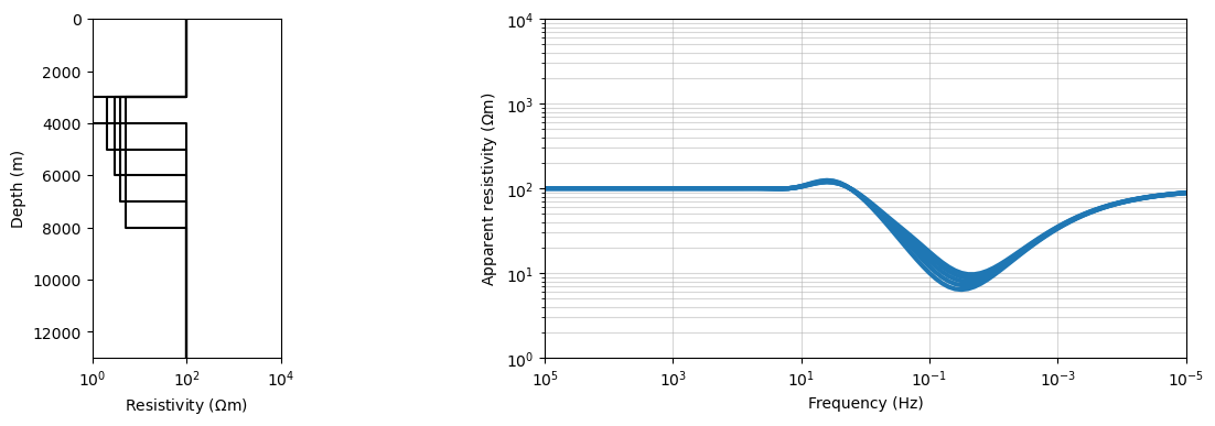
Manual fitting of the data
from mtpy import MTCollectionmc = MTCollection()
mc.open_collection("../../data/transfer_functions/yellowstone_mt_collection.h5")from ipywidgets import widgets, interact
station_names = mc.dataframe.station.values
def foo(name):
tf = mc.get_tf(name)
tf.plot_mt_response()[‘SR209’, ‘YNP05S’]
Q = interact(foo, name=widgets.Select(options=station_names, value='YNP05S'))Loading...
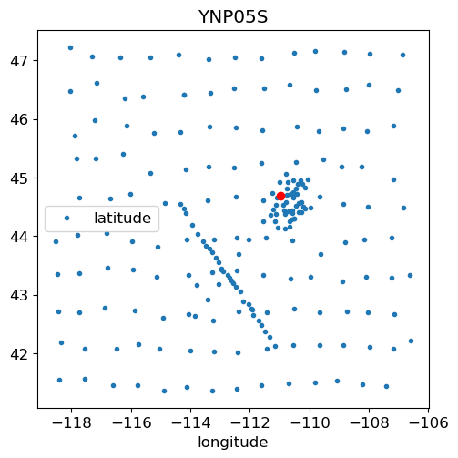
matplotlib.rcParams['font.size'] = 12name = Q.widget.kwargs['name']
tf = mc.get_tf(name)
fig, ax = plt.subplots(1,1, figsize=(5,5))
mc.dataframe.plot(x='longitude', y='latitude', marker='.', linestyle='None', ax=ax)
ax.plot(tf.longitude, tf.latitude, 'ro')
ax.set_title(name)24:10:27T17:27:17 | WARNING | line:311 |mtpy.core.mt_collection | get_tf | Found multiple transfer functions with ID YNP05S. Suggest setting survey, otherwise returning the TF from survey YSBB.
fig, ax = plt.subplots(1,1, figsize=(8, 2))
ax.loglog(tf.Z.period, tf.Z.res_det, label='det')
ax.loglog(tf.Z.period, tf.Z.res_xy, label='Zxy')
ax.loglog(tf.Z.period, tf.Z.res_yx, label='Zyx')
ax.set_xlabel("Period (s)")
ax.set_ylabel("$\\rho_a$ (Ohm-m)")
ax.legend()
ax.grid(which='both', alpha=0.5)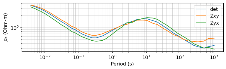
frequencies_fit = 1./tf.period
source_list_fit = []
for freq in frequencies_fit:
    source_list_fit.append(nsem.sources.Planewave(receivers_list, freq))

survey_fit = nsem.survey.Survey(source_list_fit)

simulation_fit = nsem.simulation_1d.Simulation1DRecursive(
    survey=survey_fit,
    sigmaMap=sigma_map,
    thicknessesMap=layer_map,
)
import matplotlib.gridspec as gridspec
def predict_mt_response(rho1, rho2, rho3, z, t):
model = np.log(np.r_[1./rho3, 1./rho2, 1./rho1, t, z])
pred = simulation_fit.dpred(model)
return preddef fit_mt_response(rho1, rho2, rho3, z, t):
pred = predict_mt_response(rho1, rho2, rho3, z, t)
app_res = pred.reshape((len(frequencies_fit), 2))[:,0]
fig = plt.figure(figsize=(16*0.7, 5*0.7))
gs = gridspec.GridSpec(1, 5, figure=fig)
ax0 = fig.add_subplot(gs[0, 0])
layer_thicknesses = np.array([z, t])
rho = np.r_[rho1, rho2, rho3]
plot_1d_layer_model(layer_thicknesses, rho, ax=ax0, color="k", **{'label':'True'})
ax0.set_xlabel("Resistivity ($\Omega$m)")
ax0.set_xlim(0.1, 10000)
ax = fig.add_subplot(gs[0, 2:])
ax.loglog(tf.period, tf.Z.res_det, color='C0', label='Obs.', lw=3, marker='o', linestyle='None')
ax.loglog(tf.period, app_res, color='C1', label='Pred.', lw=3)
ax.set_xlabel("Periods (s)")
ax.set_ylim(tf.Z.res_det.min()/2, tf.Z.res_det.max()*2)
ax.grid(True, which='both', alpha=0.5)
ax.set_ylabel("Apparent resistivity ($\Omega$m)")
ax.legend(bbox_to_anchor=(-0.1, 1))
ax.set_title(name)
plt.show()
# plt.tight_layout()Q_fit = interact(
fit_mt_response,
rho1=widgets.FloatLogSlider(base=10, value=np.median(tf.Z.res_det), min=-1, max=4, continuous_update=True, description="$\\rho_1$"),
rho2=widgets.FloatLogSlider(base=10, value=np.median(tf.Z.res_det), min=-1, max=4, continuous_update=True, description="$\\rho_2$"),
rho3=widgets.FloatLogSlider(base=10, value=np.median(tf.Z.res_det), min=-1, max=4, continuous_update=True, description="$\\rho_3$"),
z=widgets.FloatLogSlider(base=10, value=3000, min=0, max=5, continuous_update=True, description="$z$"),
t=widgets.FloatLogSlider(base=10, value=1000, min=0, max=5, continuous_update=True, description="$thk$"),
)Loading...
{‘rho1’: 316.2277660168379, ‘rho2’: 12.589254117941675, ‘rho3’: 316.2277660168379, ‘z’: 630.957344480193, ‘t’: 316.2277660168379}
Q_fit.widget.kwargs{'rho1': 94.8554279515094,
'rho2': 94.8554279515094,
'rho3': 94.8554279515094,
'z': 3000.0,
't': 1000.0}