Invert Yellowstone Data

from simpeg import (
    maps, utils, data, optimization, maps, regularization, 
    inverse_problem, directives, inversion, data_misfit
)
import discretize
from discretize.utils import mkvc, refine_tree_xyz
from simpeg.electromagnetics import natural_source as nsem
import numpy as np
from scipy.spatial import cKDTree
import matplotlib.pyplot as plt
from pymatsolver import Pardiso as Solver
from matplotlib.colors import LogNorm

from ipywidgets import interact, widgets
import warnings
from mtpy import MTCollection
warnings.filterwarnings("ignore", category=FutureWarning)

%%time
with MTCollection() as mc:
    mc.open_collection("../../data/transfer_functions/yellowstone_mt_collection.h5")
    out = mc.apply_bbox(*[-111.4, -109.85, 44, 45.2])
    mc.mth5_collection.tf_summary.summarize()
    mt_data=mc.to_mt_data(bounding_box=[-111.4, -109.85, 44, 45.2])

for station_id in ["YNP44S", "YNP33B", "WYYS3"]:
    mt_data.remove_station(station_id)

periods = mt_data.get_periods()

interp_periods = np.array([0.1, 1., 10, 100])
interp_mt_data = mt_data.interpolate(interp_periods, inplace=False)

1./interp_periods

interp_mt_data.compute_model_errors()
interp_mt_data.model_epsg = 32612
interp_mt_data.compute_relative_locations()

sdf = interp_mt_data.to_dataframe()

gdf = interp_mt_data.to_geo_df()

rx_loc = np.hstack(
    (mkvc(gdf.model_north.to_numpy(), 2), 
     mkvc(gdf.model_east.to_numpy(), 2),
     np.zeros((np.prod(gdf.shape[0]), 1)))
)

#frequencies = np.array([1e-1, 2])
#station_spacing = 8000
#factor_spacing = 4
#rx_x, rx_y = np.meshgrid(np.arange(0, 50000, station_spacing), np.arange(0, 50000, station_spacing))
#rx_loc = np.hstack((mkvc(rx_x, 2), mkvc(rx_y, 2), np.zeros((np.prod(rx_x.shape), 1))))
#print(rx_loc.shape)
fig, ax = plt.subplots(1,1, figsize=(5,5))
ax.plot(rx_loc[:, 0], rx_loc[:, 1], '.')
ax.set_aspect(1)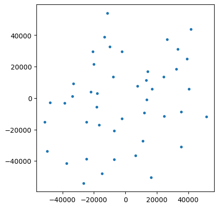

import discretize.utils as dis_utils
from discretize import TreeMesh
from geoana.em.fdem import skin_depth

def get_octree_mesh(
    rx_loc, frequencies, sigma_background, station_spacing,
    factor_x_pad=2,
    factor_y_pad=2,
    factor_z_pad_down=2,
    factor_z_core=1,
    factor_z_pad_up=1,
    factor_spacing=4,
    ):
    f_min =  frequencies.min()
    f_max =  frequencies.max()
    
    lx_pad = skin_depth(f_min, sigma_background) * factor_x_pad
    ly_pad = skin_depth(f_min, sigma_background) * factor_y_pad
    lz_pad_down = skin_depth(f_min, sigma_background) * factor_z_pad_down
    lz_core = skin_depth(f_min, sigma_background) * factor_z_core
    lz_pad_up = skin_depth(f_min, sigma_background) * factor_z_pad_up

    lx_core = rx_loc[:,0].max() - rx_loc[:,0].min()
    ly_core = rx_loc[:,1].max() - rx_loc[:,1].min()
    lx = lx_pad + lx_core + lx_pad
    ly = ly_pad + ly_core + ly_pad
    lz = lz_pad_down + lz_core + lz_pad_up
    dx = station_spacing / factor_spacing
    dy = station_spacing / factor_spacing
    dz = np.round(skin_depth(f_max, sigma_background)/4, decimals=-1)

    # Compute number of base mesh cells required in x and y
    nbcx = 2 ** int(np.ceil(np.log(lx / dx) / np.log(2.0)))
    nbcy = 2 ** int(np.ceil(np.log(ly / dy) / np.log(2.0)))
    nbcz = 2 ** int(np.ceil(np.log(lz / dz) / np.log(2.0)))
    print (dx, dy, dz)
    mesh = dis_utils.mesh_builder_xyz(
        rx_loc, 
        [dx, dy, dz],
        padding_distance=[[lx_pad, lx_pad], [ly_pad, ly_pad], [lz_pad_down, lz_pad_up]],
        depth_core=lz_core,
        mesh_type='tree'
    )
    X, Y = np.meshgrid(mesh.nodes_x, mesh.nodes_y)
    topo = np.c_[X.flatten(), Y.flatten(), np.zeros(X.size)]
    mesh = refine_tree_xyz(
        mesh, topo, octree_levels=[0, 1, 4, 4, 4], method="surface", finalize=False
    )

    mesh = refine_tree_xyz(
        mesh, rx_loc, octree_levels=[1, 0, 0], method="radial", finalize=True
    )    
    return mesh

mesh = get_octree_mesh(
    rx_loc,
    1./interp_periods,
    1e-2, 
    5000,
    factor_spacing=2,
    factor_x_pad=4,
    factor_y_pad=4
)
print(mesh.n_cells)

sigma_background = np.ones(mesh.nC) * 1e-8
ind_active = mesh.cell_centers[:,2] < 0.
sigma_background[ind_active] = 1e-2

fig = plt.figure(figsize=(10, 10))
ax = fig.add_subplot(1,2,1)
mesh.plot_slice(
    sigma_background, grid=True, normal='Z', ax=ax,
    pcolor_opts={"cmap":"turbo", "norm":LogNorm(vmin=1e-3, vmax=1)},
    grid_opts={"lw":0.1, "color":'k'}, 
    range_x=(rx_loc[:,0].min()-5000, rx_loc[:,0].max()+5000), 
    range_y=(rx_loc[:,0].min()-5000, rx_loc[:,0].max()+5000), 
    slice_loc=0.
)
ax.plot(rx_loc[:,0], rx_loc[:,1], 'ro')
ax.set_aspect(1)

ax2 = fig.add_subplot(1,2,2, sharex=ax)
mesh.plot_slice(
    sigma_background, grid=True, normal='X', ax=ax2,
    pcolor_opts={"cmap":"turbo", "norm":LogNorm(vmin=1e-4, vmax=10)},
    grid_opts={"lw":0.1, "color":'k'}, 
    range_x=(rx_loc[:,0].min()-10000, rx_loc[:,0].max()+10000), 
    range_y=(-50000, 50000*0.1)
)
ax2.plot(rx_loc[:,0], rx_loc[:,2], 'ro')
ax2.set_aspect(3)
fig.tight_layout()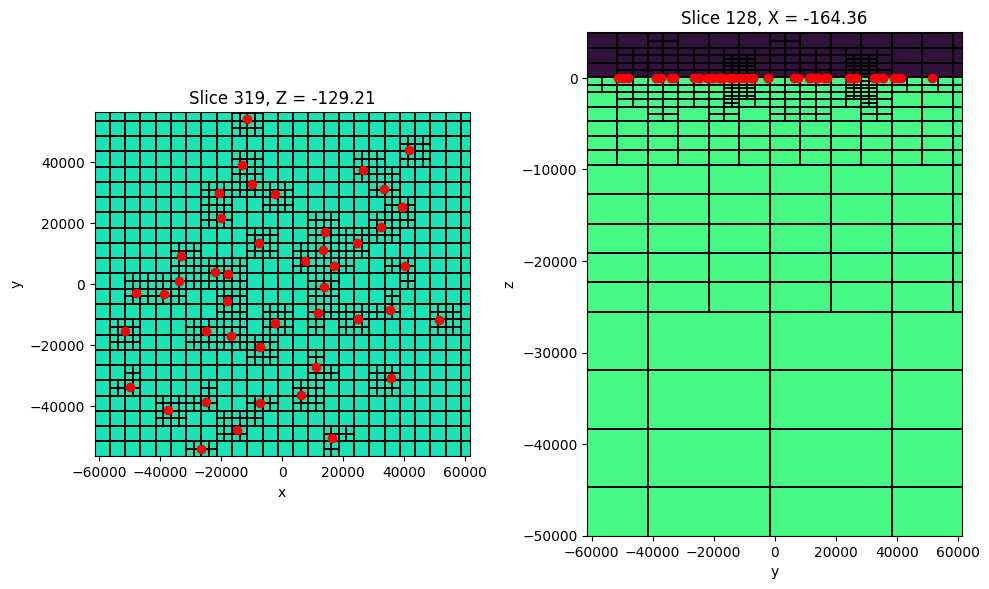

# Generate a Survey
rx_list = []
# rx_orientations_impedance = ['xy', 'yx', 'xx', 'yy']
rx_orientations_impedance = ['xy', 'yx']
for rx_orientation in rx_orientations_impedance:    
    rx_list.append(     
        nsem.receivers.PointNaturalSource(
            rx_loc, orientation=rx_orientation, component="real"
        )
    )
    rx_list.append(     
        nsem.receivers.PointNaturalSource(
            rx_loc, orientation=rx_orientation, component="imag"
        )
    )
    
# rx_orientations_tipper = ['zx', 'zy']
# for rx_orientation in rx_orientations_tipper:    
#     rx_list.append(     
#         nsem.receivers.Point3DTipper(
#             rx_loc, orientation=rx_orientation, component="real"
#         )
#     )
#     rx_list.append(
#         nsem.receivers.Point3DTipper(
#             rx_loc, orientation=rx_orientation, component="imag"
#         )
#     )
# Source list
src_list = [nsem.sources.PlanewaveXYPrimary(rx_list, frequency=f) for f in 1./interp_periods]

# Survey MT
survey = nsem.Survey(src_list)
# rx_orientations = rx_orientations_impedance + rx_orientations_tipper
rx_orientations = rx_orientations_impedance 

constant = 1./np.pi * np.sqrt(5./8.) * 10**3.5

print (constant)

frequencies = 1/interp_periods
# components = ["z_xx", "z_xy", "z_yx", "z_yy", "t_zx", "t_zy"]
# components = ["z_yx", "z_xy", "z_yy", "z_xx", "t_zy", "t_zx"]
# components = ["res_yx", "res_xy"]

# components = ["z_yx", "z_xy", "z_yy", "z_xx"]
components = ["z_yx", "z_xy"]
n_rx = rx_loc.shape[0]
n_freq = len(interp_periods)
n_component = 2
n_orientation = len(rx_orientations)

f_dict = dict([(round(ff, 5), ii) for ii, ff in enumerate(1/interp_periods)])
observations = np.zeros((n_freq, n_orientation, n_rx, n_component))
errors = np.zeros_like(observations)
for s_index, station in enumerate(gdf.station):
    station_df = sdf.loc[sdf.station == station]
    station_df.set_index("period", inplace=True)
    for row in station_df.itertuples():
        f_index = f_dict[round(1./row.Index, 5)]
        for c_index, comp in enumerate(components):
            value = getattr(row, comp)
            # print (round(1./row.Index, 5), comp, value)
            if 't' in comp:
                value *= -1
            err = getattr(row, f"{comp}_model_error") # user_set error
            observations[f_index, c_index, s_index, 0] = value.real
            observations[f_index, c_index, s_index, 1] = value.imag               
            errors[f_index, c_index, s_index, 0] = err
            errors[f_index, c_index, s_index, 1] = err       

observations[np.where(observations == 0)] = 1e-3
observations[np.isnan(observations)] = 1e-3
# errors = abs(observations) * 0.05
errors[np.where(observations == 1e-3)] = np.inf

def foo_data(i_freq, i_orientation, i_component):
    fig, ax = plt.subplots(1,1, figsize=(5, 5))
    vmin = np.min([observations[i_freq, i_orientation, :, i_component].min()])
    vmax = np.max([observations[i_freq, i_orientation, :, i_component].max()])
    out1 = utils.plot2Ddata(rx_loc, observations[i_freq, i_orientation, :, i_component], clim=(vmin, vmax), ax=ax, contourOpts={'cmap':'turbo'}, ncontour=20)
    ax.plot(rx_loc[:,0], rx_loc[:,1], 'kx')
    if i_orientation<4:
        transfer_type = "Z"
    else:
        transfer_type = "T"
    ax.set_title("Frequency={:.1e}, {:s}{:s}-{:s}".format(1./interp_periods[i_freq], transfer_type, rx_orientations[i_orientation], components[i_component]))

interact(
    foo_data,
    i_freq=widgets.IntSlider(min=0, max=n_freq-1),
    i_orientation=widgets.IntSlider(min=0, max=n_component-1), 
    i_component=widgets.IntSlider(min=0, max=n_orientation-1), 
)

constant = 1./np.pi * np.sqrt(5./8.) * 10**3.5

dobs = observations.flatten() / constant
standard_deviation = errors.flatten() / constant
dobs[np.isnan(dobs)] = 100.
standard_deviation[dobs==100.] = np.inf

# Assign uncertainties
# make data object
data_object = data.Data(survey, dobs=dobs, standard_deviation=standard_deviation)

# data_object.standard_deviation = stdnew.flatten()  # sim.survey.std
plt.semilogy(abs(data_object.dobs), '.r')
plt.semilogy(abs(data_object.standard_deviation), 'k.', ms=1)
# plt.yscale('symlog')
plt.show()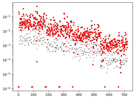

# Set the mapping
# active_map = maps.InjectActiveCells(
#     mesh=mesh, indActive=ind_active, valInactive=np.log(1e-8)
# )
# mapping = maps.ExpMap(mesh) * active_map

# True model 
m_true = np.log(sigma_background[ind_active])

# # Setup the problem object
# simulation = nsem.simulation.Simulation3DPrimarySecondary(   
#     mesh,
#     survey=survey,
#     sigmaMap=mapping,
#     sigmaPrimary=sigma_background,
#     solver=Solver

# )

mt_sims = []
mt_mappings = []
surveys = []
for i in range(len(src_list)):
    # Set the mapping
    active_map = maps.InjectActiveCells(
        mesh=mesh, indActive=ind_active, valInactive=np.log(1e-8)
    )
    mapping = maps.ExpMap(mesh) * active_map    
    survey_chunk = nsem.Survey(src_list[i])
    mt_sims.append(
        nsem.simulation.Simulation3DPrimarySecondary(    
            mesh,
            survey=survey_chunk,
            sigmaMap=maps.IdentityMap(),
            sigmaPrimary=sigma_background,
            solver=Solver
        )
    )
    surveys.append(survey_chunk)
    mt_mappings.append(mapping)
    print (f"{i}, {frequencies[i]:.1f} Hz")

from simpeg.meta import MultiprocessingMetaSimulation
parallel_sim = MultiprocessingMetaSimulation(mt_sims, mt_mappings, n_processes=4)

%%time
dpred = parallel_sim.dpred(m_true)

# data_object.standard_deviation = stdnew.flatten()  # sim.survey.std
plt.semilogy(abs(data_object.dobs), '.r')
plt.semilogy(abs(dpred) , 'k.', ms=1)
# plt.yscale('symlog')

%%time
# Optimization
opt = optimization.ProjectedGNCG(maxIter=10, maxIterCG=20, upper=np.inf, lower=-np.inf)
opt.remember('xc')
# Data misfit
dmis = data_misfit.L2DataMisfit(data=data_object, simulation=parallel_sim)
# Regularization
dz = mesh.h[2].min()
dx = mesh.h[0].min()
regmap = maps.IdentityMap(nP=int(ind_active.sum()))
reg = regularization.Sparse(mesh, active_cells=ind_active, mapping=regmap)
reg.alpha_s = 1e-8
reg.alpha_x = dz/dx
reg.alpha_y = dz/dx
reg.alpha_z = 1.

# Inverse problem
inv_prob = inverse_problem.BaseInvProblem(dmis, reg, opt)
# Beta schedule
beta = directives.BetaSchedule(coolingRate=1, coolingFactor=2)
# Initial estimate of beta
beta_est = directives.BetaEstimate_ByEig(beta0_ratio=1e0)
# Target misfit stop
target = directives.TargetMisfit()
# Create an inversion object
save_dictionary = directives.SaveOutputDictEveryIteration()
directive_list = [beta, beta_est, target, save_dictionary]
inv = inversion.BaseInversion(inv_prob, directiveList=directive_list)

# Set an intitial guess
m_0 = np.log(sigma_background[ind_active])
m_recovered = inv.run(m_0)

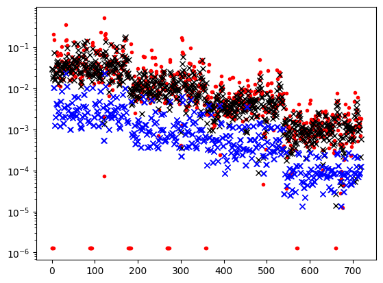
iteration = len(save_dictionary.outDict)
iteration = 2
m = save_dictionary.outDict[iteration]['m']
sigma_est = mapping*m
pred = save_dictionary.outDict[iteration]['dpred']
# DPRED = pred.reshape((n_freq, n_orientation, n_component, n_rx))
# DOBS = dpred.reshape((n_freq, n_orientation, n_component, n_rx))
# MISFIT = (DPRED-DOBS)/STD

# data_object.standard_deviation = stdnew.flatten()  # sim.survey.std
plt.semilogy(abs(data_object.dobs), '.r')
plt.semilogy(abs(pred) , 'kx')
plt.semilogy(abs(standard_deviation) , 'bx')
# plt.yscale('symlog')
# plt.semilogy(abs(data_object.standard_deviation), 'b.', ms=1)
plt.show()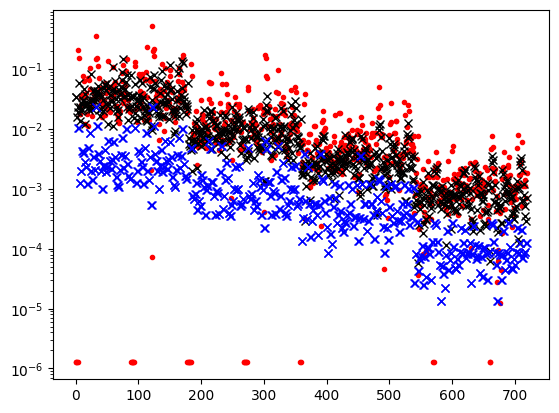

fig, ax = plt.subplots(1,1, figsize=(5, 5))
z_loc = -0.
y_loc = 0.
mesh.plot_slice(
    sigma_est, grid=True, normal='Z', ax=ax,
    pcolor_opts={"cmap":"turbo", "norm":LogNorm(vmin=5e-3, vmax=1e-1)},
    range_x=(rx_loc[:,0].min()-10000, rx_loc[:,0].max()+10000), 
    range_y=(rx_loc[:,0].min()-10000, rx_loc[:,0].max()+10000), 
    slice_loc=z_loc
)
ax.set_yticklabels([])
ax.plot(rx_loc[:,0], rx_loc[:,1], 'kx')
ax.set_aspect(1)
ax.set_xlabel("Easting (m)")
ax.set_ylabel("Northing (m)")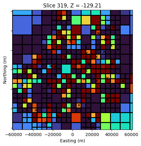

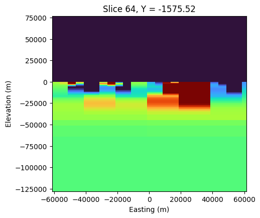
fig, ax = plt.subplots(1,1, figsize=(5, 5))
mesh.plot_slice(
    sigma_est, grid=False, normal='Y', ax=ax,
    pcolor_opts={"cmap":"turbo", "norm":LogNorm(vmin=2e-3, vmax=1e-1)},
    range_x=(rx_loc[:,0].min()-10000, rx_loc[:,0].max()+10000), 
    # range_y=(-lx_core, lx_core*0.1),
    slice_loc=y_loc
)
# ax.set_yticklabels([])
# ax.plot(rx_loc[:,0], rx_loc[:,2], 'kx')
ax.set_aspect(0.54)
ax.set_xlabel("Easting (m)")
ax.set_ylabel("Elevation (m)")

from ipywidgets import interact, widgets

# def foo_misfit(i_freq, i_orientation, i_component):
#     fig, axs = plt.subplots(1,3, figsize=(15, 5))
#     ax1, ax2, ax3 = axs

#     vmin = np.min([DOBS[i_freq, i_orientation, i_component,:].min(), DPRED[i_freq, i_orientation, i_component,:].min()])
#     vmax = np.max([DOBS[i_freq, i_orientation, i_component,:].max(), DPRED[i_freq, i_orientation, i_component,:].max()])

#     out1 = utils.plot2Ddata(rx_loc, DOBS[i_freq, i_orientation, i_component,:], clim=(vmin, vmax), ax=ax1, contourOpts={'cmap':'turbo'}, ncontour=20)
#     out2 = utils.plot2Ddata(rx_loc, DPRED[i_freq, i_orientation, i_component,:], clim=(vmin, vmax), ax=ax2, contourOpts={'cmap':'turbo'}, ncontour=20)
#     out3 = utils.plot2Ddata(rx_loc, MISFIT[i_freq, i_orientation, i_component,:], clim=(-5, 5), ax=ax3, contourOpts={'cmap':'turbo'}, ncontour=20)

#     ax.plot(rx_loc[:,0], rx_loc[:,1], 'kx')

# interact(
#     foo_misfit,
#     i_freq=widgets.IntSlider(min=0, max=n_freq-1),
#     i_orientation=widgets.IntSlider(min=0, max=n_orientation-1), 
#     i_component=widgets.IntSlider(min=0, max=n_component-1), 
# )

models = {}
models["estimated_sigma"] = sigma_est
mesh.write_vtk("yellowstone",models=models)