Now that we have an MTCollection stored in an MTH5 we can now plot interesting things. All the plotting functions can be called directly from the MTCollection object. First, let’s plot station coverage.
from pathlib import Path
from mtpy import MTCollection
%matplotlib inline
Open MTCollection
In the previous example we created a MTH5 file from existing Yellowstone data. Let’s open that file here for plotting.
mc = MTCollection()
mc.open_collection(Path().cwd().parent.parent.joinpath("data", "transfer_functions", "yellowstone_mt_collection_02.h5"))
Plot Stations
First lets plot the station coverage on a map. MTpy uses contextily if installed to get a USGS Topo map to plot the stations on to. If you want a different map, maybe imagery, just change the cx_source to what you would like. See Contextily Documentation for more details.
For geospatial plotting a method called MTCollection.to_geo_df is provided to produce a Geopandas.DataFrame object that can be used for plotting station locations. You can specify the datum if you like using the EPSG code. This is called internally in plot_stations, but good to know its there.
For now lets plot all the stations so we have an idea of the full spatial coverage.
station_plot = mc.plot_stations(map_epsg=4326, bounding_box=None)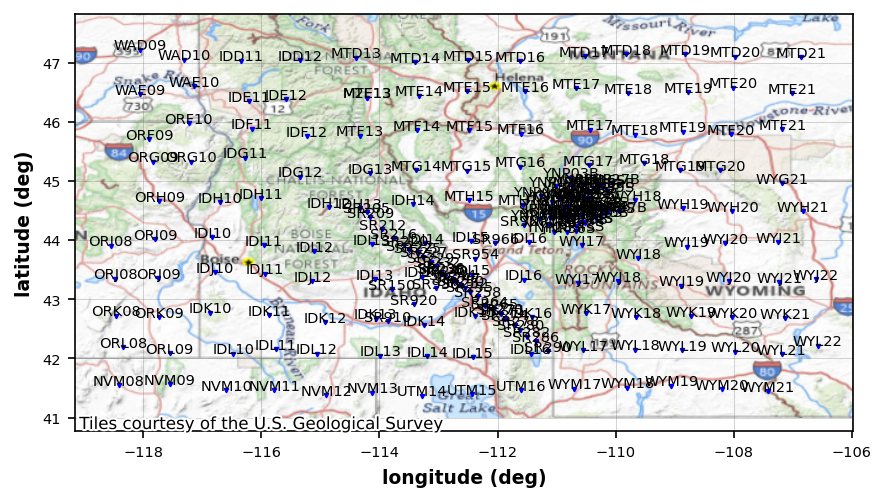
Plot Parameters
At first pass the plot is a little messy, lets update some parameters go make it look nicer.
# marker parameters
station_plot.marker_size = 10
station_plot.marker_color = (.75, 0, .1)

# station font size
station_plot.text_size = 6
station_plot.text_y_pad = .1

# redraw
station_plot.redraw_plot()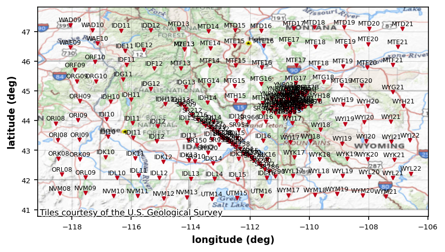
Select an area using bounding box
The dense are of stations near Yellowstone is our local target. Lets select a bounding box on initialization of plot_stations.
The bounding box needs to be (min(longitude), max(longitude), min(latitude), max(latitude))
plot_yellowstone_stations = mc.plot_stations(bounding_box=[-112, -109.5, 44, 45.75], marker_size=10, marker_color=(.75, 0, .1), text_size=6, text_y_pad=.025, fig_num=2)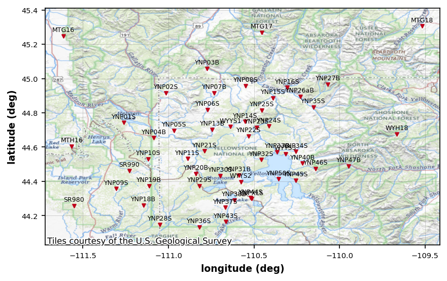
Select Stations using Working Dataframe
Another way to select stations would be to set the working_dataframe to only the “YNP” stations.
mc.working_dataframe = mc.master_dataframe[mc.master_dataframe.station.str.contains("YNP")]plot_ynp_stations = mc.plot_stations(marker_size=10, marker_color=(.75, 0, .1), text_size=6, text_y_pad=.025, fig_num=3) 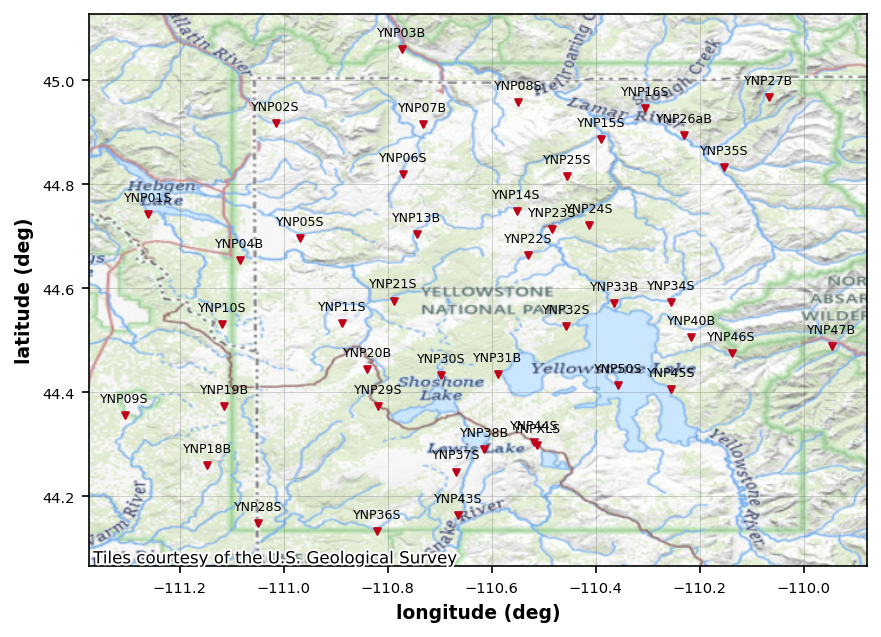
Change the Background Map
Maybe you don’t want to look at the topo, but want to look at the imagery. You can set the cx_source to something that will show imagery, though sometimes the imagery isn’t great, at least from the USGS. Other providers may have better options
import contextily as cxUSGS Imagery and Topo
plot_ynp_stations.cx_source = cx.providers.USGS.USImageryTopo
plot_ynp_stations.fig_num = 4
plot_ynp_stations.text_color = (1, 1, 1)
plot_ynp_stations.redraw_plot()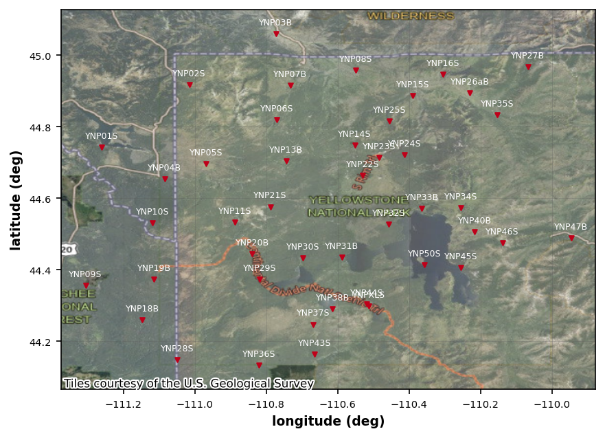
Terrain
plot_ynp_stations.cx_source = cx.providers.Esri.WorldTerrain
plot_ynp_stations.fig_num = 5
plot_ynp_stations.text_color = (0, 0, 0)
plot_ynp_stations.redraw_plot()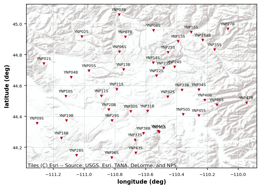
Basic Map
plot_ynp_stations.cx_source = cx.providers.Esri.WorldStreetMap
plot_ynp_stations.fig_num = 6
plot_ynp_stations.redraw_plot()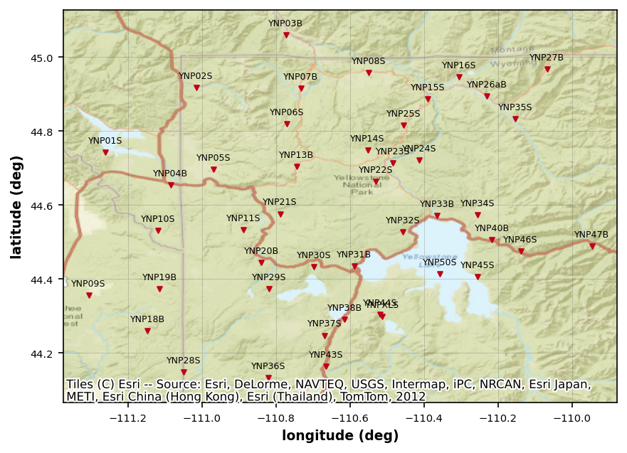
Imagery
plot_ynp_stations.cx_source = cx.providers.Esri.WorldImagery
plot_ynp_stations.fig_num = 7
plot_ynp_stations.text_color = (1, 1, 1)
plot_ynp_stations.redraw_plot()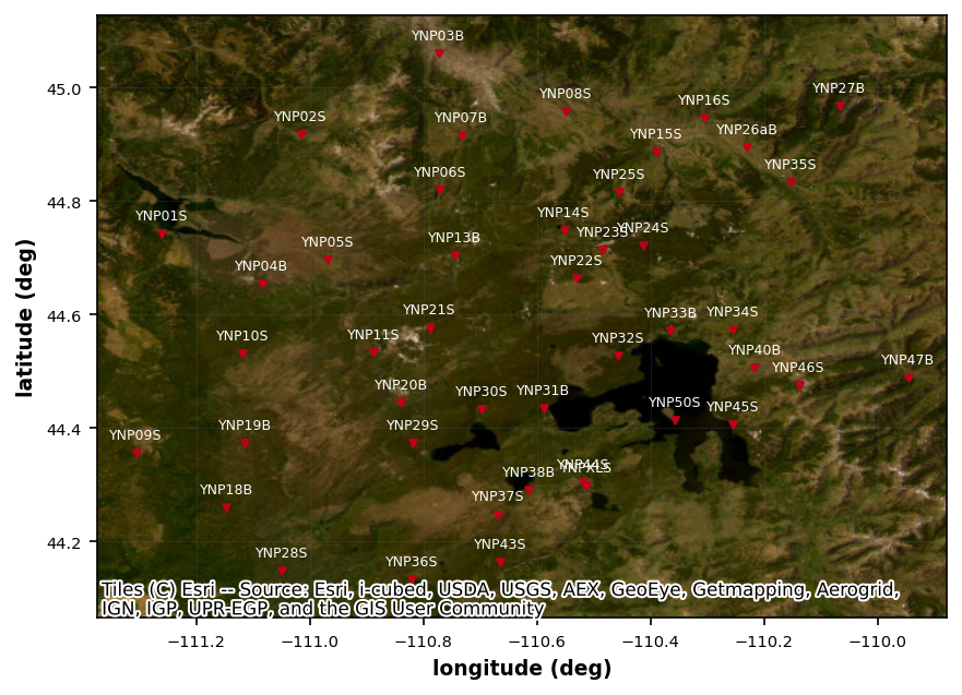
Close Collection
Remember it is important to close the collection when we are done so there are no open instances of the H5 file.
mc.close_collection()24:09:26T12:31:00 | INFO | line:777 |mth5.mth5 | close_mth5 | Flushing and closing c:\Users\jpeacock\OneDrive - DOI\Documents\GitHub\iris-mt-course-2022\data\transfer_functions\yellowstone_mt_collection_02.h5